smooth.components package
This section first explains how to create a new component and what are their generic properties. Listed below are components that can already be used in an energy system model (see examples directory for the usage of components in an energy system).
Building a component
In order to build a component, you must do the following:
- Create a subclass of the mother Component (or External Component) class.
- In the
__init__()function, define all parameters that are specific to your component, and set default values. - Consider if the component requires variable artificial costs depending on system behaviour. If it does, the method for setting the appropriate costs has to be defined in the
prepare_simulation()function of the new component. - Define any other functions that are specific to your component.
- All components built in SMOOTH must be created as oemof components to be used in the oemof model (see oemof-solph’s component list to choose the best fitting component). Then add the component to your oemof model using the
add_to_oemof_model()function, defining all of the necessary parameters. - If the states of the component need updating after each time step, specifiy these in the
update_states()function.
Artificial costs
The oemof framework always solves the system by minimizing the costs. In order to be able to control the system behaviour in a certain way, artificial costs as a concept is introduced. These costs are defined in the components and are used in the oemof model (and therefore have an effect on the cost minimization). While artificial costs are treated the same way as real costs by the oemof solver, they are being neglected in the financial evaluation at the end of the simulation. Unwanted system behaviour can be avoided by setting high (more positive) artificial costs, while the solver can be incentivised to choose a desired system behaviour by implementing lower (more negative) artificial costs.
Foreign states
Some component behaviour is dependant on so called foreign states - namely a state or attribute of another component (e.g. the artificial costs of the electricity grid can be dependant on a storage state of charge in order to fill the storage with grid electricity when the storage is below a certain threshold). While the effect of the foreign states is determined in the component itself, the mechanics on how to define the foreign states is the same for each component. Foreign states are always defined by the attributes:
- fs_component_name: string (or list of strings for multiple foreign states) of the foreign component
- fs_attribute_name: string (or list of strings for multiple foreign states) of the attribute name of the component
If a fixed value should be used as a foreign state, here fs_component_name has to be set to None and fs_attribute_name has to be set to the numerical value.
Financials
The costs and revenues are tracked for each component individually. There are three types of costs that are taken into consideration in the energy system, namely capital expenditures (CAPEX), operational expenditures (OPEX) and variable costs. The CAPEX costs are fixed initial investment costs (EUR), the OPEX costs are the yearly operational and maintenance costs (EUR/a) and the variable costs are those that are dependant on the use of the component in the system, such as the cost of buying/selling electricity from/to the grid (EUR/unit).
The financial analysis is based on annuities of the system. The CAPEX cost of a component for one year is calculated by taking into consideration both the lifetime of the given component and the interest rate, and the OPEX costs remains the same because they are already as annuities. The variable cost annuities for the components are calculated by converting the summed variable costs over the simulation time to the summed variable costs over a one year period. If the simulation time is a year, the variable cost annuities are simply the summed variable costs for a year. The below equations demonstrate how the CAPEX and variable costs are calculated. For more information on the financial analysis and the possible fitting methods for the costs, refer to the update_annuities and update_fitted_cost modules in the smooth.framework.functions package.
- \(CAPEX_{annuity}\) = CAPEX annuity [EUR/a]
- \(CAPEX\) = total CAPEX [EUR]
- \(I\) = interest rate [-]
- \(L\) = component life time [a]
- \(VC_{annuity}\) = annual variable costs [EUR/a]
- \(VC\) = total variable costs [EUR]
- \(S\) = number of simulation days [days]
Component - The mother class of all components
The generic component class is the mother class for all of the components. The parameters and functions defined here are inherited by each of the specific components.
-
class
smooth.components.component.Component¶ Bases:
objectParameters: - component (str) – component type
- name (str) – specific name of the component (must be different to other component names in the system)
- life_time (numerical) – lifetime of the component [a]
- sim_params (object) – simulation parameters such as the interval time and interest rate
- results (dict) – dictionary containing the main results for the component
- states (dict) – dictionary containing the varying states for the component
- variable_costs (numeric) – variable costs of the component [EUR/*]
- artificial_costs (numeric) – artificial costs of the component [EUR/*] (Note: these costs are not included in the final financial analysis)
- dependency_flow_costs (tuple) – flow that the costs are dependent on
- capex (dict) – capital costs
- opex (dict) – operational and maintenance costs
- variable_emissions (float) – variable emissions of the component [kg/*]
- dependency_flow_emissions (tuple) – flow that the emissions are dependent on
- op_emissions (dict) – operational emission values
- fix_emissions (dict) – fixed emission values
- fs_component_name (str) – foreign state component name
- fs_attribute_name (str) – foreign state attribute name
-
add_to_oemof_model(busses, model)¶ This function adds the specific component to the oemof energy system model and has to be defined for each component.
Parameters: - busses (dict) – Dict of the virtual buses used in the energy system
- model (oemof model) – current oemof model
Raises: NotImplementedError – NotImplementedError raised if the function is not overwritten in specific component definition.
-
check_validity()¶ This function is called immediately after the component object is created and checks if the component attributes are valid.
Raises: ValueError – Value error raised if the life time is not defined or is less than or equal to 0
-
generate_results()¶ Generates the results after the simulation.
Returns: Results for the calculated emissions, financials and annuities
-
get_costs_and_art_costs()¶ Initialize the total variable costs and art. costs [EUR/*]
Returns: The total variable costs (including artificial costs)
-
get_foreign_state_value(components, index=None)¶ Get a foreign state attribute value with the name fs_attribute_name of the component fs_component_name. If the fs_component_name is None and the fs_attribute_name set to a number, the number is given back instead.
Parameters: - components (object) – List containing each component object
- index (int, optional) – Index of the foreign state (should be None if there is only one foreign state) [-]
Returns: Foreign state value
-
prepare_simulation(components)¶ Prepares the simulation. If a component has artificial costs, this prepare_simulation function is overwritten in the specific component.
Parameters: components (list) – List containing each component object Returns: If used as a placeholder, nothing will be returned. Else, refer to specific component that uses the prepare_simulation function for further detail.
-
set_parameters(params)¶ Sets the parameters that have been defined by the user (in the model definition) in the necessary components, overwriting the default parameter values. Errors are raised if: - the given parameter is not part of the component - the dependency flows have not been defined
Parameters: params (dict ToDo: make sure of this, maybe list) – The set of parameters defined in the specific component class Raises: ValueError – Value error is raised if the parameter defined by the user is not part of the component, or dependency flows are not defined Returns: None
-
update_constraints(busses, model_to_solve)¶ Sometimes special constraints are required for the specific components, which can be written here. Else, this function is used as placeholder for components without constraints.
Parameters: - busses (dict) – Dict of the virtual buses used in the energy system
- model_to_solve – ToDo: look this up in oemof
Returns: If used as a placeholder, nothing will be returned. Else, refer to specific component that uses the update_constraints function for further detail.
-
update_flows(results, comp_name=None)¶ Updates the flows of a component for each time step.
Parameters: - results (object) – The oemof results for the given time step
- comp_name (str, optional) – The name of the component - while components can generate more than one oemof model, they sometimes need to give a custom name, defaults to None
Returns: updated flow values for each flow in the ‘flows’ dict
-
update_states(results)¶ Updates the states, used as placeholder for components without states. If a component has states, this update_states function is overwritten in the specific component.
Parameters: results (object) – oemof results object for the given time step Returns: if used as a placeholder, nothing will be returned. Else, refer to specific component that uses the update_states function for further detail.
-
update_var_costs()¶ Tracks the cost and artificial costs of a component for each time step.
Returns: New values for the updated variable and artificial costs stored in results[‘variable_costs’] and results[‘art_costs’] respectively
-
update_var_emissions()¶ Tracks the emissions of a component for each time step.
Returns: A new value for the updated emissions stored in results[‘variable_emissions’]
Air Source Heat Pump
This module represents an air source heat pump that uses ambient air and electricity for heat generation, based on oemof thermal’s component.
Scope
Air source heat pumps as a means of heat generation extract outside air and increase its temperature using a pump that requires electricity as an input. These components have the potential for the efficient utilization of energy production and distribution in a system, particularly in times of high renewable electricity production coupled with a high thermal demand.
Concept
The basis for the air source heat pump component is obtained from the oemof thermal component, in particular using the cmpr_hp_chiller function to pre-calculate the coefficient of performance. For further information on how this function works, visit oemof thermal’s readthedocs site [1].
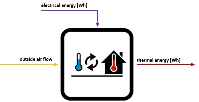
Fig.1: Simple diagram of an air source heat pump.
References
[1] oemof thermal (2019). Compression Heat Pumps and Chillers, Read the Docs: https://oemof-thermal.readthedocs.io/en/latest/compression_heat_pumps_and_chillers.html
-
class
smooth.components.component_air_source_heat_pump.AirSourceHeatPump(params)¶ Bases:
smooth.components.component.ComponentParameters: - name (str) – unique name given to the air source heat pump component
- bus_el (str) – electrical bus input of the heat pump
- bus_th – thermal bus output of the heat pump
- power_max (numerical) – maximum heating output [W]
- life_time (numerical) – life time of the component
- csv_filename (str) – csv filename containing the desired timeseries, e.g. ‘my_filename.csv’
- csv_separator (str) – separator of the csv file, e.g. ‘,’ or ‘;’ (default is ‘,’)
- column_title (str or int) – column title (or index) of the timeseries, default is 0
- path (str) – path where the timeseries csv file can be located
- temp_threshold_icing (numerical) – temperature below which icing occurs [K]
- temp_threshold_icing_C (numerical) – converts to degrees C for oemof thermal function [C]
- temp_high (numerical) – output temperature from the heat pump [K]
- temp_high_C (numerical) – converts to degrees C for oemof thermal function [C]
- temp_high_C_list (list) – converts to list for oemof thermal function
- temp_low (numerical) – ambient temperature [K]
- temp_low_C (numerical) – converts to degrees C for oemof thermal function [C]
- quality_grade (numerical) – quality grade of heat pump [-]
- mode (str) – can be set to heat_pump or chiller
- factor_icing (numerical) – COP reduction caused by icing [-]
- set_parameters – updates parameter default values (see generic Component class)
- cops (numerical) – coefficient of performance (pre-calculated by oemof thermal function)
-
add_to_oemof_model(busses, model)¶ Creates an oemof Transformer component from information given in the AirSourceHeatPump class, to be used in the oemof model
Parameters: - busses (dict) – virtual buses used in the energy system
- model (oemof model) – current oemof model
Returns: oemof component
Battery
This module represents a stationary battery.
Scope
Batteries are crucial in effectively integrating high shares of renewable energy electricity sources in diverse energy systems. They can be particularly useful for off-grid energy systems, or for the management of grid stability and flexibility. This flexibility is provided to the energy system by the battery in times where the electric consumers cannot.
Concept
The battery component has an electricity bus input and output, where factors such as the charging and discharging efficiency, the loss rate, the C-rates and the depth of discharge define the electricity flows.
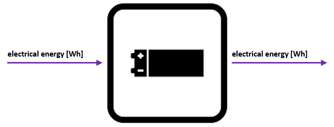
Fig.1: Simple diagram of a battery storage.
Wanted storage level
Within this component, there is the possibility to choose a wanted storage level that the energy system should try to maintain when it feasibly can. If the state of charge level wanted is defined, the variable artificial costs change depending on whether the storage level is above or below the desired value. If the battery level is too low, the artificial costs of storing electricity into the battery can be reduced and the costs of extracting electricity from the battery can be increased to incentivise the system to maintain the wanted storage level.
Maximum chargeable/dischargeable energy
The maximum power [W] going in to or out of the battery are dependent on the C-rate and the capacity:
- \(P_{in,max}\) = maximum power flowing from bus to battery [W]
- \(E_{cap}\) = battery capacity [Wh]
- \(C_{r,charge}\) = C-Rate for charging [W/Wh]
- \(P_{out,max}\) = maximum power flowing from battery to bus [W]
- \(C_{r,discharge}\) = C-Rate for discharging [W/Wh]
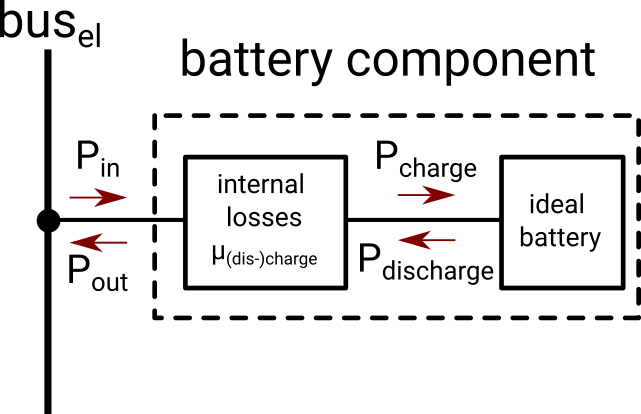
Fig.2: Diagram of the battery component including losses.
The amount of energy that the battery will be charged or discharged takes the energy losses during the (dis-)charging process into account:
- \(P_{charge,max}\) = maximum chargeable power at the battery [W]
- \(\mu_{charge}\) = charging efficiency [-]
- \(P_{discharge,max}\) = maximum dischargeable power at the battery [W]
- \(\mu_{discharge}\) = discharging efficiency [-]
-
class
smooth.components.component_battery.Battery(params)¶ Bases:
smooth.components.component.ComponentParameters: - name (str) – unique name given to the battery component
- bus_in_and_out (str) – electricity bus the battery is connected to
- battery_capacity (numerical) – battery capacity (assuming all the capacity can be used) [Wh]
- soc_init (numerical) – initial state of charge [-]
- efficiency_charge (numerical) – charging efficiency [-]
- efficiency_discharge (numerical) – discharging efficiency [-]
- loss_rate (numerical) – loss rate [%/day]
- symm_c_rate (boolean) – flag to indicate if the c-rate is symmetrical
- c_rate_symm (numerical) – C-Rate for charging and discharging (only used if symm_c_rate==True) [-/h]
- c_rate_charge (numerical) – C-Rate for charging [-/h]
- c_rate_discharge (numerical) – C-Rate for discharging [-/h]
- soc_min (numerical) – minimal state of charge [-]
- life_time (numerical) – life time of the component [a]
- vac_in (numerical) – normal variable artificial costs for charging (in) the battery [EUR/Wh]
- vac_out (numerical) – normal variable artificial costs for discharging (out) the battery [EUR/Wh]
- soc_wanted (numerical) – if a soc level is set as wanted, the vac_low costs apply if the capacity is below that level [Wh]
- vac_low_in (numerical) – variable artificial costs that apply (in) if the capacity level is below the wanted capacity level [EUR/Wh]
- vac_low_out (numerical) – variable artificial costs that apply (in) if the capacity level is below the wanted capacity level [EUR/Wh]
- set_parameters(params) (function) – updates parameter default values (see generic Component class)
- soc (numerical) – state of charge [-]
- p_in_max (numerical) – max. chargeable power [W]
- p_out_max (numerical) – max. dischargeable power [W]
- loss_rate – adjusted loss rate to chosen timestep [%/timestep]
- current_vac (list) – current artificial costs for input and output [EUR/Wh]
-
add_to_oemof_model(busses, model)¶ Creates an oemof Generic Storage component from the information given in the Battery class, to be used in the oemof model.
Parameters: - busses (dict) – virtual buses used in the energy system
- model (oemof model) – current oemof model
Returns: oemof component
-
check_flows()¶ Checks if there are flows in and out of the battery and if so triggers an AssertionError
Raises: ValueError if flows in and out of the battery at the same time are detected
-
prepare_simulation(components)¶ Prepares the simulation by setting the appropriate artificial costs
Parameters: components (list) – List containing each component object (unused in this component)
-
update_flows(results, comp_name=None)¶ Update flow values for each flow in the ‘flows’ dict of results
Parameters: - results (object) – The oemof results for the given time step
- comp_name (str, optional) – The name of the component - while components can generate more than one oemof model, they sometimes need to give a custom name, defaults to None
-
update_states(results)¶ Updates the states of the battery component for each time step
Parameters: results (object) – oemof results for the given time step Returns: updated state values for each state in the ‘state’ dict
Biogas Converter
This module represents the conversion of a biogas input in m3 to kg, where the biogas composition is defined.
Scope
The biogas converter component is a virtual component, so would not be found in a real life energy system. Its purpose is to transform a biogas bus with m3 units into a biogas bus with kg units. This might be necessary because the Biogas SMR PSA component, for instance, requires a biogas input in kg.
Concept
The biogas converter component takes in a biogas bus as an input and outputs a different biogas bus. The composition of the biogas is defined, as well as the energy content per m3 of biogas.
Biogas composition
The user can determine the desired composition of biogas by stating the percentage share of methane and carbon dioxide in the gas. The default share is chosen to be 75.7% methane, 24.3% carbon dioxide [1]. The lower heating value (LHV) of methane is 13.9 kWh/kg [2], and the molar masses of methane and carbon dioxide are 0.01604 kg/mol and 0.04401 kg/mol, respectively. The method used to calculate the LHV of biogas is the same as in the Gas Engine CHP Biogas component, and the equation used is as follows:
- \(LHV_{Bg}\) = heating value of biogas [kWh/kg]
- \(CH_{4_{share}\) = proportion of methane in biogas [-]
- \(M_{CH_{4}}\) = molar mass of methane [kg/mol]
- \(CO_{2_{share}}\) = proportion of carbon dioxide in biogas [-]
- \(M_{CO_{2}}\) = molar mass of carbon dioxide [kg/mol]
- \(LHV_{CH_{4}}\) = heating value of methane [kWh/kg]
References
[1] Braga, L. B. et.al. (2013). Hydrogen production by biogas steam reforming: A technical, economic and ecological analysis, Renewable and Sustainable Energy Reviews. [2] Linde Gas GmbH (2013). Rechnen Sie mit Wasserstoff. Die Datentabelle.
-
class
smooth.components.component_biogas_converter.BiogasConverter(params)¶ Bases:
smooth.components.component.ComponentParameters: - name (str) – unique name given to the biogas converter component
- bg_in (str) – input biogas bus
- bg_out (str) – output biogas bus
- ch4_share (numerical) – proportion of methane in biogas [-]
- co2_share (numerical) – proportion of carbon dioxide in biogas [-]
- kwh_1m3_bg (numerical) – energy content in 1m3 biogas [kWh/m3]
- set_parameters(params) (function) – updates parameter default values (see generic Component class)
- mol_mass_ch4 (numerical) – molar mass of methane [kg/mol]
- mol_mass_co2 (numerical) – molar mass of carbon dioxide [kg/mol]
- heating_value_ch4 (numerical) – heating value of methane [kWh/kg]
- heating_value_bg (numerical) – heating value of biogas [kWh/kg]
-
add_to_oemof_model(busses, model)¶ Creates an oemof Transformer component from the information given in the BiogasConverter class, to be used in the oemof model
Parameters: - busses (dict) – virtual buses used in the energy system
- model (oemof model) – current oemof model
Returns: oemof component
Biogas Steam Methane Reformer with Pressure Swing Adsorption
This module represents a biogas steam methane reformer that produces hydrogen, combined with the pressure swing adsorption process to produce 99.9 % pure hydrogen.
Scope
The primary production of hydrogen is currently from the process of steam methane reforming (SMR), using natural gas as the feed material. Biogas can be used as an alternative feed material, which has a similar composition to natural gas. The utilisation of biogas can be beneficial due to biogas being a renewable resource, and its usage can lead to less methane emissions in the atmosphere. Pressure swing adsorption (PSA) is a process used in combination with SMR to purify the output hydrogen stream to a level of approximately 99.9 % [1].
Concept
The biogas SMR PSA component takes in a biogas bus and electricity bus as inputs, with a hydrogen bus output. An oemof Transformer component is chosen for this component, and is illustrated in Figure 1.
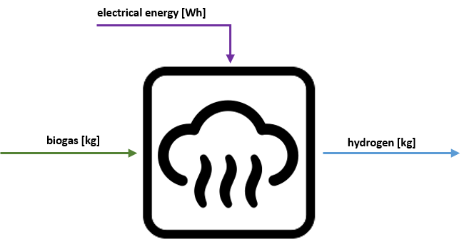
Fig.1: Simple diagram of a biogas steam methane reformer
Hydrogen production from SMR
The amount of hydrogen produced in SMR from the chosen composition of biogas is calculated based on results from [2]. The default amount of input fuel required to produce 1kg of H2 is 45.977 kWh, and using this value along with the LHV of biogas, the amount of biogas required to produce 1kg of H2 is determined:
- \(Bg_{kg H2}\) = biogas required to produce one kg H2 [kg]
- \(fuel_{kg H2}\) = specific fuel consumption per kg of H2 produced [kWh/kg]
- \(LHV_{Bg}\) = heating value of biogas [kWh/kg]
In order to calculate how much hydrogen will be produced in SMR from the input amount of biogas, the conversion efficiency is calculated:
- \(smr_{eff}\) = conversion efficiency of biogas to hydrogen in SMR process [-]
Hydrogen purification with PSA
The hydrogen produced in SMR contains many impurities such as carbon dioxide and carbon monoxide, and these can be removed using the PSA process. The default efficiency of the PSA process is taken to be 90 % [3], so the overall efficiency of the SMR PSA process is determiend by:
- \(overall_{eff}\) = overall efficiency of biogas to 99.9 % pure hydrogen in SMR and PSA process [-]
- \(psa_{eff}\) = efficiency of inpure to pure hydrogen is PSA process [-]
Energy consumption
The default energy consumption of the combined SMR and PSA process per kg of H2 produced is 5.557 kWh/kg [1]. Thus the energy consumption per kg of biogas used is:
- \(EC_{kg Bg}\) = energy required per kg of biogas used [Wh/kg]
References
[1] Song, C. et.al. (2015). Optimization of steam methane reforming coupled with pressure swing adsorption hydrogen production process by heat integration, Applied Energy. [2] Minh, D. P. et.al. (2018). Hydrogen Production From Biogas Reforming: An Overview of Steam Reforming, Dry Reforming, Dual Reforming and Tri-Reforming of Methane. [3] Air Liquide Engineering & Construction (2021). Druckwechseladsorption Wasserstoffreinigung Rückgewinnung und Reinigung von Wasserstoff durch PSA.
-
class
smooth.components.component_biogas_smr_psa.BiogasSmrPsa(params)¶ Bases:
smooth.components.component.ComponentParameters: - name (str) – unique name given to the biogas SMR PSA component
- bus_bg (str) – biogas bus that is the input of the component
- bus_el (str) – electricity bus that is the input of the component
- bus_h2 (str) – 99.9 % pure hydrogen bus that is the output of the component
- life_time (numerical) – lifetime of the component [a]
- input_max (numerical) – maximum biogas input per interval [kg/*]
- fuel_kwh_1kg_h2 (numerical) – specific fuel consumption per kg of H2 produced [kWh/kg]
- psa_eff (numerical) – efficiency of the PSA process [-]
- energy_cnsmp_1kg_h2 (numerical) – specific energy consumption of the combined SMR and PSA process in terms of hydrogen production [kWh/kg]
- set_parameters(params) (function) – updates parameter default values (see generic Component class)
- smr_psa_eff (numerical) – total efficiency of biogas to 99.9 % pure hydrogen in SMR and PSA process [-]
- energy_cnsmp_1kg_bg (numerical) – specific energy consumption of the combined SMR and PSA process in terms of biogas consumption [Wh/kg]
-
add_to_oemof_model(busses, model)¶ Creates an oemof Transformer component using the information given in the BiogasSteamReformer class, to be used in the oemof model
Parameters: - busses (dict) – buses used in the energy system
- model (oemof model) – current oemof model
Returns: oemof component
-
prepare_simulation(components)¶ Prepares the simulation by calculating the specific compression energy
Parameters: components (list) – list containing each component object Returns: the specific compression energy [Wh/kg]
Compressor (Hydrogen)
This module represents a hydrogen compressor.
Scope
A hydrogen compressor is used in energy systems as a means of increasing the pressure of hydrogen to suitable levels for feeding into other components in the system or satisfying energy demands.
Concept
The hydrogen compressor is powered by electricity and intakes a low pressure hydrogen flow while outputting a hgh pressure hydrogen flow. The efficiency of the compressor is assumed to be 88.8%.
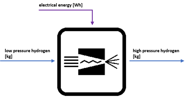
Fig.1: Simple diagram of a hydrogen compressor.
Specific compression energy
The specific compression energy is calculated by first obtaining the compression ratio:
- \(p_{ratio}\) = compression ratio
- \(p_{out}\) = outlet pressure [bar]
- \(p_{in}\) = inlet pressure [bar]
Then the output temperature is calculated, and the initial assumption for the polytropic exponent is assumed to be 1.6:
- \(T_{out}\) = output temperature [K]
- \(T_{in}\) = input temperature [K]
- \(n_{init}\) = initial polytropic exponent
Then the temperature ratio is calculated:
- \(T_{ratio}\) = temperature ratio
Then the polytropic exponent is calculated:
The compressibility factors of the hydrogen entering and leaving the compressor is then calculated using interpolation considering varying temperature, pressure and compressibility factor values (see the calculate_compressibility_factor function). The real gas compressibility factor is calculated using these two values as follows:
- \(Z_{real}\) = real gas compressibility factor
- \(Z_{in}\) = compressibility factor on entry
- \(Z_{out}\) = compressibility factor on exit
Thus the specific compression work is finally calculated:
- \(c_{w_{1}}\) = specific compression work [kJ/kg]
- \(\mu\) = compression efficiency
- \(R_{H_{2}}\) = hydrogen gas constant
Finally, the specific compression work is converted into the amount of electrical energy required to compress 1 kg of hydrogen:
- \(c_{w_{2}}\) = specific compression energy [Wh/kg]
-
class
smooth.components.component_compressor_h2.CompressorH2(params)¶ Bases:
smooth.components.component.ComponentParameters: - name (str) – unique name given to the compressor component
- bus_h2_in (str) – lower pressure hydrogen bus that is an input of the compressor
- bus_el (str) – electricity bus that is an input of the compressor
- bus_h2_out (str) – higher pressure hydrogen bus that is the output of the compressor
- m_flow_max (numerical) – maximum mass flow through the compressor [kg/h]
- life_time (numerical) – life time of the component [a]
- temp_in (numerical) – temperature of hydrogen on entry to the compressor [K]
- efficiency (numerical) – overall efficiency of the compressor [-]
- set_parameters(params) (function) – updates parameter default values (see generic Component class)
- spec_compression_energy (numerical) – specific compression energy (electrical energy needed per kg H2) [Wh/kg]
- R (numerical) – gas constant (R) [J/(K*mol)]
- Mr_H2 (numerical) – molar mass of H2 [kg/mol]
- R_H2 (numerical) – specific gas constant for H2 [J/(K*kg)]
-
add_to_oemof_model(busses, model)¶ Creates an oemof Transformer component using the information given in the CompressorH2 class, to be used in the oemof model
Parameters: - busses (dict) – virtual buses used in the energy system
- model (oemof model) – current oemof model
Returns: oemof component
-
prepare_simulation(components)¶ Prepares the simulation by calculating the specific compression energy
Parameters: components (list) – list containing each component object Returns: the specific compression energy [Wh/kg]
-
update_states(results)¶ Updates the states in the compressor component
Parameters: results (object) – oemof results object for the given time step Returns: updated values for each state in the ‘states’ dict
-
smooth.components.component_compressor_h2.calculate_compressibility_factor(p_in, p_out, temp_in, temp_out)¶ Calculates the compressibility factor through interpolation.
Parameters: - p_in (numerical) – inlet pressure [bar]
- p_out (numerical) – outlet pressure [bar]
- temp_in (numerical) – inlet temperature of the hydrogen [K]
- temp_out (numerical) – outlet temperature of the hydrogen [K]
Electric Heater
A simple electric heater component that converts electricity to heat is created through this module.
Scope
Electric heaters can convert electricity into heat directly with a high efficiency, which can be useful in energy systems with large quantitites of renewable electricity production as well as a heat demand that must be satisfied.
Concept
A simple oemof Transformer component is used to convert the electricity bus into a thermal bus, with a constant efficiency of 98% applied [1].
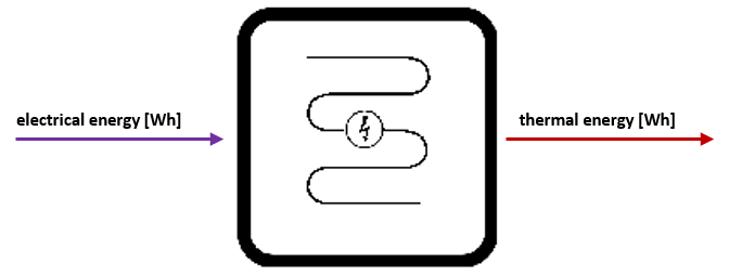
Fig.1: Simple diagram of an electric heater.
References
[1] Meyers, S. et.al. (2016). Competitive Assessment between Solar Thermal and Photovoltaics for Industrial Process Heat Generation, International Solar Energy Society.
-
class
smooth.components.component_electric_heater.ElectricHeater(params)¶ Bases:
smooth.components.component.ComponentParameters: - name (str) – unique name given to the electric heater component
- bus_el (str) – electricity bus that is the input of the electric heater
- bus_th (str) – thermal bus that is the output of the electric heater
- power_max (numerical) – maximum thermal output [W]
- life_time (numerical) – life time of the component [a]
- efficiency (float (0-1)) – constant efficiency of the heater [-]
- set_parameters(params) (function) – updates parameter default values (see generic Component class)
-
add_to_oemof_model(busses, model)¶ Creates an oemof Transformer component from the information given in the ElectricHeater class, to be used in the oemof model
Parameters: - busses (dict) – virtual buses used in the energy system
- model (oemof model) – current oemof model
Returns: oemof component
Electrolyzer (alkaline)
This module represents an alkaline electrolyzer that exhibits non-linear behaviour.
Scope
The conversion of electricity into hydrogen can be done through the process of electrolysis. There is a widespread use of alkaline water electrolyzers in dynamic energy systems (involving hydrogen production) due to their simplicity, and providing the electrolyzer with electricity from renewable sources can result in sustainable hydrogen production.
Concept
The alkaline electrolyser intakes an electricity flow and outputs a hydrogen flow. The behaviour of the alkaline electrolyzer is non-linear, which is demonstrated through the use of oemof’s Piecewise Linear Transformer component.
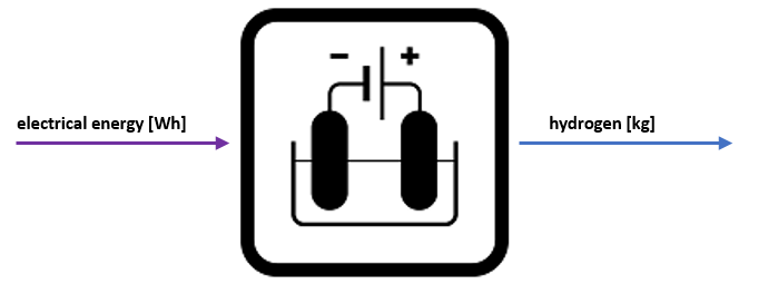
Fig.1: Simple diagram of an alkaline electrolyzer.
Maximum power
In order to make it possible to define the maximum power of the electrolyser, the number of cells required in the electrolyser is adjusted accordingly. This is achieved by checking how many cells lead to the maximum power at maximum temperature.
Maximum hydrogen production
The maximum amount of hydrogen that can be produced in one time step is determined by the following equation:
- \(H_{2,max}\) = maximum hydrogen produced in one time step [kg]
- \(J_{max}\) = maximum current density [A/cm^2]
- \(A_{cell}\) = size of cell surface [cm²]
- \(t\) = interval time
- \(z_{cell}\) = number of cells per stack
- \(F\) = faraday constant F [As/mol]
- \(M_{H_{2}}\) = molar mass M_H2 [g/mol]
Hydrogen production
Initially, the breakpoints are set up for the electrolyzer conversion of electricity to hydrogen. The breakpoint values for the electric energy are taken in ten evenly spaced incremental steps from 0 to the maximum energy, and the hydrogen production and resulting electrolyzer temperature at each breakpoint is eventually determined.
First, the current density at each breakpoint is calculated (see get_electricity_by_power function). Using this value, the hydrogen mass produced is calculated:
- \(H_2\) = hydrogen produced in one time step [kg]
- \(I\) = current [A]
Varying temperature
The new temperature of the electrolyzer is calculated using Newton’s law of cooling. The temperature to which the electrolyzer will heat up to depends on the given current density. Here, linear interpolation is used:
- \(T_{aim}\) = temperature to which the electrolyser is heating up, depending on current density [K]
- \(T_{min}\) = minimum temperature of electrolyzer [K]
- \(T_{max}\) = maximum temperature of electrolyzer [K]
- \(J\) = current density [A/cm²]
- \(J_{T_{max}}\) = current density at maximum temperature [A/cm²]
- \(T_{new}\) = new temperature of electrolyzer [K]
- \(T_{new}\) = new temperature of electrolyzer [K]
- \(T_{old}\) = old temperature of electrolyzer [K]
- \(t\) = interval time [min]
Additional calculations
For more in depth information on how parameters such as the current density or reversible voltage are calculated, see inside the component for the necessary functions.
-
class
smooth.components.component_electrolyzer.Electrolyzer(params)¶ Bases:
smooth.components.component.ComponentParameters: - name (str) – unique name given to the electrolyser component
- bus_el (str) – electricity bus that is the input of the electrolyser
- bus_h2 (str) – hydrogen bus that is the output of the electrolyser
- power_max (numerical) – maximum power of the electrolyser [W]
- pressure (numerical) – pressure of hydrogen in the system [Pa]
- fs_pressure (numerical) – pressure of hydrogen in the system, to be used in other components [bar]
- temp_init (numerical) – initial electrolyser temperature [K]
- life_time (numerical) – life time of the component [a]
- fitting_value_exchange_current_density (numerical) – fitting parameter exchange current density [A/cm²]
- fitting_value_electrolyte_thickness (numerical) – thickness of the electrolyte layer [cm]
- temp_min (numerical) – minimum temperature of the electrolyzer (completely cooled down) [K]
- temp_max (numerical) – highest temperature the electrolyser can be [K]
- cur_dens_max (numerical) – maximal current density given by the manufacturer [A/cm^2]
- cur_dens_max_temp (numerical) – current density at which the maximal temperature is reached [A/cm^2]
- area_cell (numerical) – size of the cell surface [cm²]
- set_parameters(params) (function) – updates parameter default values (see generic Component class)
- interval_time (numerical) – interval time [min]
-
add_to_oemof_model(busses, model)¶ Creates an oemof Transformer component from the information given in the Electrolyzer class, to be used in the oemof model
Parameters: - busses (dict) – virtual buses used in the energy system
- model (oemof model) – current oemof model
Returns: oemof component
-
conversion_fun_ely(ely_energy)¶ Gives out the hydrogen mass values for the electric energy values at the breakpoints
Parameters: ely_energy (numerical) – electric energy values at the breakpoints Returns: The according hydrogen production value [kg]
-
ely_voltage_u_act(cur_dens, temp)¶ Describes the activity losses within the electolyzer
Parameters: - cur_dens (numerical) – current density [A/cm²]
- temp (numerical) – temperature [K]
Returns: activation voltage for this node [V]
-
ely_voltage_u_ohm(cur_dens, temp)¶ Takes into account two ohmic losses, one being the # resistance of the electrolyte itself (resistanceElectrolyte) and # other losses like the presence of bubbles (resistanceOther)
Parameters: - cur_dens (numerical) – current density [A/cm²]
- temp (numerical) – temperature [K]
Returns: cell voltage loss due to ohmic resistance [V]
-
ely_voltage_u_rev(temp)¶ Calculates the reversible voltage taking two parts into consideration: the first part takes into account changes of the reversible cell voltage due to temperature changes, the second part due to pressure changes
Parameters: temp – temperature [K] Returns: reversible voltage [V]
-
get_cell_temp(cur_dens)¶ Calculates the electrolyzer temperautre for the following time step
Parameters: cur_dens (numerical) – given current density [A/cm²] Returns: new electrolyzer temperature [K]
-
get_electricity_by_power(power, this_temp=None)¶ Calculates the current density for a given power
Parameters: - power (numerical) – current power the electrolyzer is operated with [kW]
- this_temp (numerical) – temperature of the electrolyzer [K]
Returns: current density [A/cm²]
-
get_mass_and_temp(energy_used)¶ Calculates the mass of hydrogen produced along with the resulting temperature of the electrolyzer for a certain energy
Parameters: energy_used (numerical) – energy value for the next time step [kWh] Returns: produced hydrogen [kg] and the resulting electrolyzer temperature [K]
-
get_mass_produced_by_current_state(cur_dens)¶ Calculates the hydrogen mass produced by a given current density
Parameters: cur_dens (numerical) – given current density [A/cm²] Returns: hydrogen mass produced [kg]
-
update_nonlinear_behaviour()¶ Updates the nonlinear behaviour of the electrolyser in terms of hydrogen production, as well as the resulting temperature of the electrolyser
-
update_states(results)¶ Updates the states of the electrolyser component for each time step
Parameters: results (object) – oemof results for the given time step Returns: updated state values for each state in the ‘state’ dict
Electrolyzer Waste Heat (alkaline)
This module is created as a subclass of the alkaline Electrolyzer module with the inclusion of a waste heat model.
Scope
The significance of including the heat generation from an electrolyzer in an energy system is that this heat can be utilized for other means (e.g. contributing towards a heat demand) as opposed to wasted. This will be particularly important with the implementation of large scale electrolyzers, where there is the potential to recover large quantities of energy.
Concept
In this component, it is assumed that the alkaline electrolyzer consists of a cylindrical cell stack along with two cylindrical gas separators. It is further assumed that:
- The cell stack height consists of the cells plus two ends. The height of the end of the stack which is not part of the cells has a dependence on the diameter of the cell. The ratio is taken as 7:120 [1]
- The height of an individual cell is in a ratio of 1:75.5 with the cell diameter [2]
- The overall surface area exposed by the gas separators and the pipe communicating them is in a ratio of 1:0.42 with the surface area of the stack [3]

Fig.1: Simple diagram of an alkaline electrolyzer with waste heat.
The alkaline electrolyzer with waste heat intakes an electrical flow and outputs hydrogen and thermal energy flows. The behaviour of the electrolyzer waste heat model is non-linear, which is demonstrated through the use of oemof’s Piecewise Linear Transformer component.
Waste heat
The waste heat equation is derived from the heat balance equation, found in [3]. From this equation, it is shown that the change of the electrolyzer temperature comes from the electrical power input dissipated as heat, without the inclusion of the heat losses to the environment, the heat removed by the cooling water, and the sum of the enthalpy leaving the system with the hydrogen and oxygen streams and the enthalpy gained from the deionized water to warm up the electrolyzer from ambient to operating temperature [3]:
#ToDo: sort out this equation including derivatives etc.
For the waste heat model in SMOOTH, the heat balance is assumed for stationary conditions. This is because the model only applies when the maximum temperature is reached, and this temperature is then kept constant because of the removal of the waste heat from the system.
The waste heat, which is removed from the electrolyzer by the cooling water, is calculated using the following equation, based on [3]:
- \(Q_{W}\) = waste heat
- \(Q_{gen}\) = internal heat generation
- \(Q_{L}\) = heat losses to the environment
- \(L\) = latent heat
- \(S\) = sensible heat
Internal heat generation
The internal heat generation within an electrolyzer is as a result of a greater energy supply to the electrolyzer than is required . This is necessary for reaching high water electrolysis rates [3]. The internal heat gemeration is calculated as follows:
- \(E_{sup}\) = total energy supply to the electrolyzer
- \(H_{2,prod}\) = the amount of hydrogen produced
- \(HHV_{H_{2}}\) = the higher heating value of hydrogen
Heat losses
In order to calculate the heat losses to the environment, the heat transfer coefficient is first calculated based on [3]. It should be noted that the following equation is specifically to determine the heat transfer coefficient for horizontal cylinders, and since the parts of the alkaline have a cylindrical shape, this equation is used for the alkaline electrolyzer component:
The heat losses are then calculated taking into consideration the heat transfer coefficient, the total surface area of the main parts of the electrolyzer (the cell stack and the gas separators) and the temperature difference between the surface of the electrolyzer and the ambient temperature [3]. The equation is as follows:
- \(A_{sep}\) = total surface area of the gas separators
- \(T_{sep}\) = separator surface temperature
- \(T_{amb}\) = ambient temperature
- \(A_{stack}\) = total surface area of the cell stack
- \(T_{stack}\) = cell stack surface temperature
Sensible and latent heat
Sensible heat
The sensible heat removed from the system within the \(H_2\) and \(O_2\) streams, as well as the sensible heat required to warm the deionized water from ambient temperature to the stack operating temperature, must be considered when determining the total waste heat. From the known mass of produced hydrogen along with the molar masses of \(H_2\) and \(O_2\), the mass of produced oxygen is determined:
- \(m_{O_{2}}\) = mass of oxygen stream
- \(m_{H_{2}}\) = mass of hydrogen stream
- \(M_{O_{2}}\) = molar mass of oxygen
- \(M_{H_{2}}\) = molar mass of hydrogen
The mass of \(H_2O\) is then determined as follows:
- \(m_{H_{2O}}\) = mass of water
Thus, the sensible heat is calculated using mass and specific heat:
- \(c_{p,H_{2}O}\) = specific heat of water
- \(\Delta T\) = the temperature change between the ambient and electrolyzer temperature
- \(c_{p,H_{2}}\) = specific heat of hydrogen
- \(c_{p,O_{2}}\) = specific heat of oxygen
Latent heat
The latent heat is neglected since the mass of \(H_{2O}\) vapor (leaving the system with the oxygen and hydrogen streams) is neglected.
Piecewise Linear Transformer
Currently, the piecewise linear transformer component in oemof can only represent a one-to-one transformation with a singular input and a singular output. Thus, in order to represent the non-linear behaviour of the alkaline electrolyser in the energy system, two oemof components are created for the hydrogen and thermal outputs individually, with a constraint that the electric input flows into each component must always be equal. In this way, the individual oemof components behave as one component.
References
[1] De Silva, Y.S.K. (2017). Design of an Alkaline Electrolysis Stack, University of Agder. [2] Vogt, U.F. et al. (2014). Novel Developments in Alkaline Water Electrolysis, Empa Laboratory of Hydrogen and Energy. [3] Dieguez, P.M. et al. (2008). Thermal Performance of a commercial alkaline water electrolyser: Experimental study and mathematical modeling, Int. J. Hydrogen Energy.
-
class
smooth.components.component_electrolyzer_waste_heat.ElectrolyzerWasteHeat(params)¶ Bases:
smooth.components.component_electrolyzer.ElectrolyzerParameters: - param_bus_th (dict) – inclusion of the thermal bus in the parameters dictionary, which was not included in the electrolyzer mother class
- bus_th (str) – thermal bus that is the output of the electrolyzer
- set_parameters(params) (function) – updates parameter default values (see generic Component class)
- interval_time (numerical) – interval time [min]
- energy_max (numerical) – maximum energy that the electrolyzer can use in one time step [Wh]
- c_p_H2 (numerical) – specific heat of hydrogen at constant pressure [J/(kg*K)]
- c_p_O2 (numerical) – specific heat of oxygen at constant pressure [J/(kg*K)]
- c_p_H2O (numerical) – specific heat of water at constant pressure [J/(kg*K)]
- diameter_cell (numerical) – diameter of the electrolyzer cell [m]
- stack_end_height (numerical) – height of the two stack ends that are not part of the cells, from the perspective of the total stack height [m]
- height_cell (numerical) – height of an individual cell in relation to the cell diameter [m]
- height_stack (numerical) – total stack height, which is calculated by taking the cell stack plus the two additional ends of the stack into consideration [m]
- area_stack (numerical) – external surface area of the electrolyser stack under the assumption that it is cylindrical [m^2]
- area_separator (numerical) – overall surface area exposed by the gas separators and the pipe communicating them [m^2]
- model_h2 (oemof model) – model created with regards to the hydrogen produced by the electrolyser
- model_th (oemof model) – model created with regards to the thermal energy produced by the electrolyser
-
add_to_oemof_model(busses, model)¶ Creates two separate oemof Piecewise Linear Transformer components for the hydrogen and thermal production of the electrolyser from information given in the ElectrolyserWasteHeat class, to be used in the oemof model
Parameters: - busses (dict) – virtual buses used in the energy system
- model (model) – oemof model containing the hydrogen production and thermal energy production of the electrolyser
Returns: the oemof electrolyzer and electrolyzer thermal components
-
conversion_fun_ely(ely_energy)¶ Gives out the hydrogen mass values for the electric energy values at the breakpoints
Parameters: ely_energy (numerical) – electric energy values at the breakpoints Returns: The according hydrogen production value [kg]
-
conversion_fun_thermal(ely_energy)¶ Gives out the thermal energy values for the electric energy values at the breakpoints
Parameters: ely_energy (numerical) – The electric energy values at the breakpoints Returns: The according thermal energy production value [Wh]
-
get_waste_heat(energy_used, h2_produced, new_ely_temp)¶ Approximates waste heat production based on calculations of internal heat generation, heat losses to the environment and the sensible and latent heat removed from the system
Parameters: - energy_used (numerical) – energy consumed by the electrolyser [kWh]
- h2_produced (numerical) – hydrogen produced by the electrolyser [kg]
- new_ely_temp (numerical) – resulting temperature of the electrolyser [K]
Returns: resulting waste heat produced by the electrolyser [kWh]
-
sensible_and_latent_heats(mass_H2, new_ely_temp)¶ Calculates the sensible and latent heat that has been removed with the hydrogen and oxygen streams leaving the system.
Parameters: - mass_H2 (numerical) – mass of hydrogen [kg]
- new_ely_temp (numerical) – resulting temperature of the electrolyser [K]
Returns: values for the sensible and latent heat
-
update_constraints(busses, model_to_solve)¶ Set a constraint so that the electric inflow of the hydrogen producing and the thermal part are always the same (which is necessary while the piecewise linear transformer cannot have two outputs yet and therefore the two parts need to be separate components).
Parameters: - busses (dict) – virtual buses used in the energy system
- model_to_solve (model) – oemof model that will be solved
-
update_flows(results)¶ Updates the flows of the electrolyser waste heat components for each time step.
Parameters: results (object) – oemof results for the given time step Returns: updated flow values for each flow in the ‘flows’ dict
-
update_nonlinear_behaviour()¶ Updates the nonlinear behaviour of the electrolyser in terms of hydrogen and thermal energy (waste heat) production, as well as the resulting temperature of the electrolyser
Energy Demand from CSV
This module represents generic energy demands, which are created through this class by the importation of CSV files.
Scope
The final energy demand component must be satisified by the energy system in the simulations/optimizations.
Concept
The generic energy demand component has one input (the bus is specified by the user), and it requires a demand time series in the form of a CSV file. Optionally, this time series can be created by oemof’s demandlib package [1]. This module uses oemof’s Sink component.
References
[1] oemof Team (2016). demandlib documentation, https://demandlib.readthedocs.io/en/latest/.
-
class
smooth.components.component_energy_demand_from_csv.EnergyDemandFromCsv(params)¶ Bases:
smooth.components.component.ComponentEnergy demand components are created through this class by importing csv files.
Parameters: - name (str) – unique name given to the energy demand component
- nominal_value (numerical) – value that the timeseries should be multipled by, default is 1
- csv_filename – csv filename containing the desired demand timeseries e.g. ‘my_demand_filename.csv’
- csv_separator (str) – separator of the csv file e.g. ‘,’ or ‘;’, default is ‘,’
- column_title (str or int) – column title (or index) of the timeseries, default is 0
- path (str) – path where the timeseries csv file can be located
- bus_in (str) – virtual bus that enters the energy demand component (e.g. the hydrogen bus)
- set_parameters(params) (function) – updates parameter default values (see generic Component class)
- data (pandas dataframe) – dataframe containing data from timeseries
-
add_to_oemof_model(busses, model)¶ Creates an oemof Sink component from the information given in the EnergyDemandFromCSV class, to be used in the oemof model.
Parameters: - busses (dict) – virtual buses used in the energy system
- model (oemof model) – current oemof model
Returns: oemof component
Energy Source from CSV
General energy source components are created through this class by importing csv files.
Scope
The energy source components usually represent the various means of renewable energy production in the energy system, which should be efficiently utilised (and sometimes scaled) to avoid excessive energy losses.
Concept
The energy source component is suitable for any energy type once the output bus has been defined as well as a time series in the form of a CSV file, which can be created through oemof’s windpowerlib or pvlib, for example [1][2].
References
[1] oemof Team (2016). windpowerlib documentation, https://windpowerlib.readthedocs.io/en/stable/. [2] pvlib Team (2020). pvlib documentation, https://pvlib-python.readthedocs.io/en/v0.7.2/.
-
class
smooth.components.component_energy_source_from_csv.EnergySourceFromCsv(params)¶ Bases:
smooth.components.component.ComponentParameters: - name (str) – unique name given to the energy source component
- nominal_value (numerical) – value that the timeseries should be multiplied by, default is 1
- csv_filename (str) – csv filename containing the desired timeseries, e.g. ‘my_filename.csv’
- csv_separator (str) – separator of the csv file, e.g. ‘,’ or ‘;’ (default is ‘,’)
- column_title (str or int) – column title (or index) of the timeseries, default is 0
- path (str) – path where the timeseries csv file can be located
- bus_out (str) – virtual bus that leaves the energy source component (e.g. the electricity bus)
- set_parameters(params) (function) – updates parameter default values (see generic Component class)
- data (pandas dataframe) – dataframe containing data from timeseries
-
add_to_oemof_model(busses, model)¶ Creates an oemof Source component from the information given in the EnergySourceFromCSV class, to be used in the oemof model.
Parameters: - busses (dict) – virtual buses used in the energy system
- model (oemof model) – current oemof model
Returns: oemof component
Fuel cell CHP
This module represents a combined heat and power (CHP) system with a fuel cell, using hydrogen to generate electricity and heat.
Scope
The importance of a fuel cell CHP component in dynamic energy systems is its potential to enable better sector coupling between the electricity and heating sectors, thus less dependence on centralised power systems by offering the ability for localised energy supply [1].
Concept
The fuel cell CHP has a hydrogen bus input along with an electrical bus and thermal bus output. The behaviour of the fuel cell CHP component is non-linear, which is demonstrated through the use of oemof’s Piecewise Linear Transformer component.
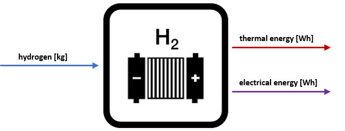
Fig.1: Simple diagram of a fuel cell CHP.
Efficiency
The efficiency curves for both electrical and thermal energy output according to nominal load which are considered for the fuel cell CHP component are displayed in Figure 2. From the breakpoints, the electrical and thermal production based on the hydrogen consumption and variable efficiency can be obtained. The piecewise linear representation that is actually used in the SMOOTH component is shown in the left image, and the approximated efficiency curve is shown in the right image.
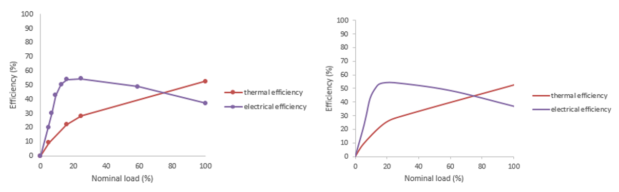
Fig.2: Piecewise and approximated efficiency of a fuel cell CHP.
Electrical and thermal energy production
In order to calculate the electrical and thermal energy production for each load point, first the maximum hydrogen input is calculated:
- \(H_{2,max}\) = maximum hydrogen input per timestep [kg]
- \(P_{max}\) = maximum electrical output power [W]
- \(\mu_{elec_{max}}\) = electrical efficiency at full load [-]
Then the load break points for both the electrical and thermal components are converted into how much hydrogen is consumed at each load break point according to the maximum hydrogen input per time step:
- \(bp_{H_{2},el,i}\) = ith electrical break point in terms of hydrogen consumption [kg]
- \(bp_{load,el,i}\) = ith electrical break point in terms of nominal load [-]
- \(bp_{H_{2},th,i}\) = ith thermal break point in terms of hydrogen consumption [kg]
- \(bp_{load,th,i}\) = ith thermal break point in terms of nominal load [-]
From these hydrogen consumption values, the absolute electrical and thermal energy produced at each break point is calculated:
- \(E_{el,i}\) = ith absolute electrical energy value [Wh]
- \(\mu_{el,i}\) = ith electrical efficiency [-]
- \(E_{th,i}\) = ith absolute thermal energy value [Wh]
- \(\mu_{th,i}\) = ith thermal efficiency [-]
Piecewise Linear Transformer
Currently, the piecewise linear transformer component in oemof can only represent a one-to-one transformation with a singular input and a singular output. Thus, in order to represent the non-linear fuel cell CHP in the energy system, two oemof components are created for the electrical and thermal outputs individually, with a constraint that the hydrogen input flows into each component must always be equal. In this way, the individual oemof components behave as one component.
References
[1] P.E. Dodds et.al. (2015). Hydrogen and fuel cell technologies for heat: A review, International journal of hydrogen energy.
-
class
smooth.components.component_fuel_cell_chp.FuelCellChp(params)¶ Bases:
smooth.components.component.ComponentParameters: - name (str) – unique name given to the fuel cell CHP component
- bus_h2 (str) – hydrogen bus that is the input of the CHP
- bus_el (str) – electricity bus that is the output of the CHP
- bus_th (str) – thermal bus that is the output of the CHP
- power_max (numerical) – maximum electrical output power [W]
- life_time (numerical) – lifetime of the component [a]
- set_parameters(params) (function) – updates parameter default values (see generic Component class)
- heating_value_h2 (numerical) – heating value of hydrogen [kWh/kg]
- bp_load_el (list) – electrical efficiency load break points [-]
- bp_eff_el (list) – electrical efficiency break points [-]
- bp_load_th (list) – thermal efficiency load break points [-]
- bp_eff_th (list) – thermal efficiency break points [-]
- h2_input_max (numerical) – maximum hydrogen input that leads to maximum electrical energy in Wh [kg]
- bp_h2_consumed_el (list) – converted electric load points according to maximum hydrogen input per time step [kg]
- bp_h2_consumed_th (list) – converted thermal load points according to maximum hydrogen input per time step [kg]
- bp_energy_el (list) – absolute electrical energy values over the load points [Wh]
- bp_energy_th (list) – absolute thermal energy values over the load points [Wh]
- bp_h2_consumed_el_half (list) – half the amount of hydrogen that is consumed [kg]
- bp_h2_consumed_th_half (list) – half the amount of hydrogen that is consumed [kg]
- model_el (model) – electric model to set constraints later
- model_th (model) – thermal model to set constraints later
-
add_to_oemof_model(busses, model)¶ Creates two separate oemof Piecewise Linear Transformer components for the electrical and thermal production of the fuel cell CHP from information given in the FuelCellCHP class, to be used in the oemof model
Parameters: - busses (dict) – virtual buses used in the energy system
- model (model) – oemof model containing the electrical energy production and thermal energy production of the fuel cell CHP
Returns: tuple of electric and thermal oemof components
-
get_el_energy_by_h2(h2_consumption)¶ Gets the electrical energy produced by the according hydrogen consumption value.
Parameters: h2_consumption – hydrogen consumption value [kg] Returns: according electrical energy value [Wh]
-
get_th_energy_by_h2(h2_consumption)¶ Gets the thermal energy produced by the according hydrogen consumption value.
Parameters: h2_consumption – hydrogen consumption value [kg] Returns: according thermal energy value [Wh]
-
update_constraints(busses, model_to_solve)¶ Set a constraint so that the hydrogen inflow of the electrical and the thermal part are always the same (which is necessary while the piecewise linear transformer cannot have two outputs yet and therefore the two parts need to be separate components).
Parameters: - busses (dict) – virtual buses used in the energy system
- model_to_solve (model) – The oemof model that will be solved
-
update_flows(results)¶ Updates the flows of the fuel cell CHP components for each time step.
Parameters: results (object) – The oemof results for the given time step Returns: updated flow values for each flow in the ‘flows’ dict
Gas Engine CHP Biogas
A combined heat and power (CHP) plant with a gas engine, using biogas to generate electricity and heat is created through this class.
Scope
Biogas CHPs play a significant role in renewable energy systems by using biogas, which has been produced from organic waste material, as a fuel source to produce both electricity and heat. The utilisation of biogas CHPs is beneficial for sector coupling and the minimisation of methane emissions as a result of using up the biogas.
Concept
The biogas CHP component requires a biogas bus input in order to output an electrical and a thermal bus, and oemof’s Piecewise Linear Transformer component is chosen to represent the nonlinear efficiencies of the biogas CHP. The method used in this component is similar to the fuel cell CHP component.
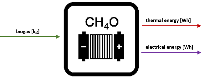
Fig.1: Simple diagram of a biogas gas engine CHP.
Biogas composition
The user can determine the desired composition of biogas by stating the percentage share of methane and carbon dioxide in the gas (the default is 50-50 % share). The lower heating value (LHV) of methane is 13.9 kWh/kg [1], and the molar masses of methane and carbon dioxide are 0.01604 kg/mol and 0.04401 kg/mol, respectively. The gas composition is given as a mole percentage, and this percentage is transformed into a mass percentage. Finally, the heating value of the biogas is found by multiplying the mass percentage with the LHV of methane, which is demonstrated below:
- \(LHV_{Bg}\) = heating value of biogas [kWh/kg]
- \(CH_{4_{share}\) = proportion of methane in biogas [-]
- \(M_{CH_{4}}\) = molar mass of methane [kg/mol]
- \(CO_{2_{share}}\) = proportion of carbon dioxide in biogas [-]
- \(M_{CO_{2}}\) = molar mass of carbon dioxide [kg/mol]
- \(LHV_{CH_{4}}\) = heating value of methane [kWh/kg]
Efficiency
The electrical and thermal production from the CHP is determined by variable efficiencies according to nominal load, and the efficiency curves used in the component can be seen in Figure 2. The piecewise linear representation that is actually used in the SMOOTH component is shown in the left image, and the approximated efficiency curve is shown in the right image.
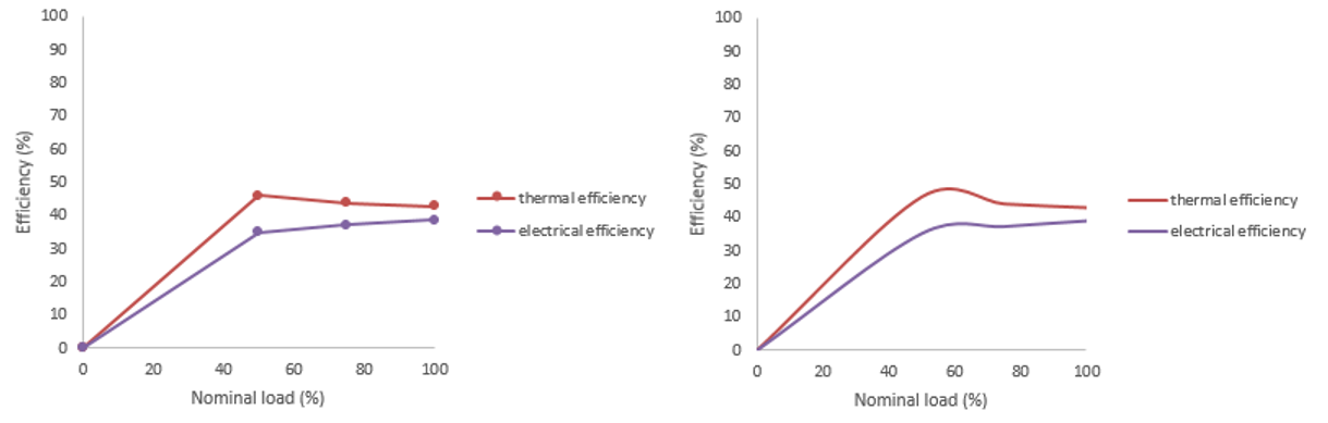
Fig.2: Piecewise and approximated efficiency of biogas gas engine CHP.
Electrical and thermal energy production
The maximum biogas input is initially calculated so that the electrical and thermal energy production for each load point can be calculated:
- \(Bg_{max}\) = maximum biogas input per timestep [kg]
- \(P_{max}\) = maximum electrical output power [W]
- \(\mu_{elec_{max}}\) = electrical efficiency at full load [-]
Then the load break points for both the electrical and thermal components are converted into how much biogas is consumed at each load break point according to the maximum biogas input per time step:
- \(bp_{Bg,el,i}\) = ith electrical break point in terms of biogas consumption [kg]
- \(bp_{load,el,i}\) = ith electrical break point in terms of nominal load [-]
- \(bp_{Bg,th,i}\) = ith thermal break point in terms of biogas consumption [kg]
- \(bp_{load,th,i}\) = ith thermal break point in terms of nominal load [-]
From these biogas consumption values, the absolute electrical and thermal energy produced at each break point is calculated:
- \(E_{el,i}\) = ith absolute electrical energy value [Wh]
- \(\mu_{el,i}\) = ith electrical efficiency [-]
- \(E_{th,i}\) = ith absolute thermal energy value [Wh]
- \(\mu_{th,i}\) = ith electrical efficiency [-]
Piecewise Linear Transformer
As stated in the fuel cell CHP component, two seperate oemof components for the electrical and thermal production of the biogas CHP must be created, but they still behave as one component by setting a constraint that the biogas input flows into the two components are always equal.
References
[1] Linde Gas GmbH (2013). Rechnen Sie mit Wasserstoff. Die Datentabelle.
-
class
smooth.components.component_gas_engine_chp_biogas.GasEngineChpBiogas(params)¶ Bases:
smooth.components.component.ComponentParameters: - name (str) – unique name given to the biogas gas engine CHP component
- bus_bg (str) – biogas bus input of the CHP
- bus_el (str) – electrical bus input of the CHP
- bus_th (str) – thermal bus input of the CHP
- power_max (numerical) – maximum electrical output power [W]
- ch4_share (numerical) – proportion of methane in biogas [-]
- co2_share (numerical) – proportion of carbon dioxide in biogas [-]
- set_parameters(params) (function) – updates parameter default values (see generic Component class)
- heating_value_ch4 (numerical) – heating value of methane [kWh/kg]
- mol_mass_ch4 (numerical) – molar mass of methane [kg/mol]
- mol_mass_co2 (numerical) – molar mass of carbon dioxide [kg/mol]
- heating_value_bg (numerical) – heating value of biogas [kWh/kg]
- bp_load_el (list) – electrical efficiency load break points [-]
- bp_eff_el (list) – electrical efficiency break points [-]
- bp_load_th (list) – thermal efficiency load break points [-]
- bp_eff_th (list) – thermal efficiency break points [-]
- bg_input_max (numerical) – maximum biogas input that leads to the maximum electrical energy in Wh [kg]
- bp_bg_consumed_el (list) – converted electric load points according to maximum hydrogen input per time step [kg]
- bp_bg_consumed_th (list :param bp_energy_el: absolute electrical energy values over the load points [Wh]) – converted thermal load points according to maximum hydrogen input per time step [kg]
- bp_energy_th (list) – absolute thermal energy values over the load points [Wh]
- bp_bg_consumed_el_half (list) – half the amount of biogas that is consumed [kg]
- bp_bg_consumed_th_half (list) – half the amount of biogas that is consumed [kg]
- model_el (model) – electric model to set constraints later
- model_th (model) – thermal model to set constraints later
-
add_to_oemof_model(busses, model)¶ Creates two separate oemof Piecewise Linear Transformer components for the electrical and thermal production of the biogas CHP from information given in the GasEngineChpBiogas class, to be used in the oemof model
Parameters: - busses (dict) – virtual buses used in the energy system
- model (model) – oemof model containing the electrical energy production and thermal energy production of the biogas CHP
Returns: tuple of electric and biogas oemof components
-
get_electrical_energy_by_bg(bg_consumption)¶ Gets the electrical energy produced by the according biogas production value.
Parameters: bg_consumption – biogas production value [kg] Returns: according electrical energy value [Wh]
-
get_thermal_energy_by_bg(bg_consumption)¶ Gets the thermal energy produced by the according biogas production value.
Parameters: bg_consumption – biogas production value [kg] Returns: according thermal energy value [Wh]
-
update_constraints(busses, model_to_solve)¶ Set a constraint so that the biogas inflow of the electrical and the thermal part are always the same (which is necessary while the piecewise linear transformer cannot have two outputs yet and therefore the two parts need to be separate components).
Parameters: - busses –
- model_to_solve (model) – The oemof model that will be solved
-
update_flows(results)¶ Updates the flows of the biogas CHP components for each time step.
Parameters: results (object) – The oemof results for the given time step Returns: updated flow values for each flow in the ‘flows’ dict
Gate
A gate component is created to transform a specific bus into a more general bus.
Scope
The gate component is a virtual component, so would not be found in a real life energy system, but is used in the framework as a means of transforming a specific bus into a more general bus. As an example, it could be useful in an energy system to initially differentiate between the electricity buses coming out of each renewable energy source, but at some point in the system it could become more useful to have only one generic electricity bus defined.
Concept
An oemof Transformer component is used to convert the chosen input bus into the chosen output bus, with a limitation on the value that can be transformed per timestep by the defined maximum input parameter. Applying an efficiency to the conversion of the input bus to the output bus is optional, with the default value set to 100%.
-
class
smooth.components.component_gate.Gate(params)¶ Bases:
smooth.components.component.ComponentParameters: - name (str) – unique name given to the gate component
- max_input (numerical) – maximum value that the gate can intake per timestep
- bus_in (str) – bus that enters the gate component
- bus_out (str) – bus that leaves the gate component
- efficiency (numerical) – efficiency of the gate component
- set_parameters(params) (function) – updates parameter default values (see generic Component class)
-
add_to_oemof_model(busses, model)¶ Creates an oemof Transformer component from information given in the Gate class, to be used in the oemof model
Parameters: - busses (dict) – virtual buses used in the energy system
- model (oemof model) – current oemof model
Returns: oemof component
H2 Refuel Cooling System
A component that represents the cooling system in a refuelling station is created through this class.
Scope
As part of the hydrogen refuelling station, a cooling system is required to precool high pressure hydrogen before it is dispensed into the vehicle’s tank. This is in order to prevent the tank from overheating.
Concept
An oemof Sink component is used which has one electrical bus input that represents the electricity required to power the cooling system.
Fig.1: Simple diagram of a hydrogen refuel cooling system.
The required electricity supply for the cooling system per timestep is calculated by the following equation:
- \(E_{elec,i}\) = electrical energy required for the ith timestep [Wh]
- \(D_{H_{2},i}\) = hydrogen demand for the ith timestep [kg]
- \(E_{spec}\) = specific energy required relative to the demand [kJ/kg]
- \(E_{standby}\) = standby energy required per timestep [kJ/h]
The default specific energy is chosen to be 730 kJ/kg, and the standby energy is chosen to be 8100 kJ/h [find source]. Furthermore, this cooling system component is only necessary if the hydrogen is compressed over 350 bar e.g. to 700 bar for passenger cars.
-
class
smooth.components.component_h2_refuel_cooling_system.H2RefuelCoolingSystem(params)¶ Bases:
smooth.components.component.ComponentParameters: - name (str) – unique name given to the H2 refuel cooling system component
- bus_el (str) – electricity bus that is the input of the cooling system
- nominal_value (numerical) – value that the timeseries should be multiplied by, default is 1
- csv_filename (str) – csv filename containing the desired timeseries, e.g. ‘my_filename.csv’
- csv_separator (str) – separator of the csv file, e.g. ‘,’ or ‘;’ (default is ‘,’)
- column_title (str or int) – column title (or index) of the timeseries, default is 0
- path (str) – path where the timeseries csv file can be located
- cool_spec_energy (numerical) – energy required to cool the refuelling station [kJ/kg]
- standby_energy (numerical) – required standby energy [kJ/h]
- life_time (numerical) – life time of the component [a]
- number_of_units – number of units installed
- set_parameters(params) (function) – updates parameter default values (see generic Component class)
- data (pandas dataframe) – dataframe containing data from timeseries
- electrical_energy (numerical) – electrical energy required for each hour [Wh]
-
add_to_oemof_model(busses, model)¶ Creates an oemof Sink component from information given in the H2RefuelCoolingSystem class, to be used in the oemof model
Parameters: - busses (dict) – virtual buses used in the energy system
- model (oemof model) – current oemof model
Returns: oemof component
H2 CHP
This module represents another combined heat and power (CHP) system that uses hydrogen to generate electricity and heat. This module is comparable to the Fuel Cell CHP module, but using different efficiencies that are based on real life data.
Scope
The importance of a hydrogen CHP component in dynamic energy systems is its potential to enable better sector coupling between the electricity and heating sectors, thus less dependence on centralised power systems by offering the ability for localised energy supply [1].
Concept
The H2 CHP component has a hydrogen bus input and electrical and thermal bus outputs. Similarly to the fuel cell CHP component, the behaviour of the H2 CHP is non-linear and represented by oemof’s Piecewise Linear Transformer component.
Fig.1: Simple diagram of an H2 CHP.
Efficiency
The efficiency of the CHP is assumed to be constant
For more detailed information, visit Fuel cell CHP
-
class
smooth.components.component_h2_chp.H2Chp(params)¶ Bases:
smooth.components.component.Component:param
-
add_to_oemof_model(busses, model)¶ Creates a non-linear oemof Transformer component to be used in the oemof model
The CHP has to be modelled as two components because the piecewise linear transformer does not accept 2 outputs yet.
Parameters: - busses (dict) – virtual buses used in the energy system
- model (oemof model) – current oemof model
Returns: tuple of electric and thermal oemof components
-
get_electrical_energy_by_h2(h2_consumption)
-
get_thermal_energy_by_h2(h2_consumption)
-
update_constraints(busses, model_to_solve)¶ Sometimes special constraints are required for the specific components, which can be written here. Else, this function is used as placeholder for components without constraints.
Parameters: - busses (dict) – Dict of the virtual buses used in the energy system
- model_to_solve – ToDo: look this up in oemof
Returns: If used as a placeholder, nothing will be returned. Else, refer to specific component that uses the update_constraints function for further detail.
-
update_flows(results)¶ Updates the flows of a component for each time step.
Parameters: - results (object) – The oemof results for the given time step
- comp_name (str, optional) – The name of the component - while components can generate more than one oemof model, they sometimes need to give a custom name, defaults to None
Returns: updated flow values for each flow in the ‘flows’ dict
-
PEM Electrolyzer
Polymer electrolyte membrane (PEM) electrolyzer agents are created through this class.
Scope
Despite being less mature in the development phase than alkaline electrolysis, thus having higher manufacturing costs, PEM electrolysis has advantages such as quick start-up times, simple maintenance and composition, as well as no dangers of corrosion [1]. If the manufacturing costs of PEM electrolyzers can be reduced by economy of scale, these electrolyzers have the potential to be crucial components in a self-sufficient renewable energy system.
Concept
The PEM electrolyzer is modelled using oemof’s Piecewise Linear Transformer components, and the component as a whole represents the intake of electricity to produce hydrogen and waste heat as a by-product.
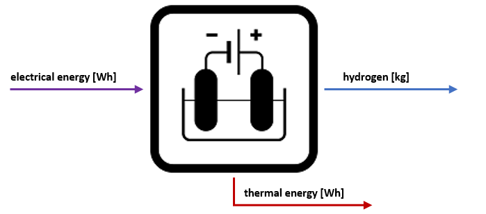
Fig.1: Simple diagram of a PEM electrolyzer.
Efficiency
The amount of hydrogen and waste heat production is dependant on variable efficiencies according to nominal load, as displayed in Figure 2. The piecewise linear representation that is actually used in the SMOOTH component is shown in the left image, and the approximated efficiency curve is shown in the right image.
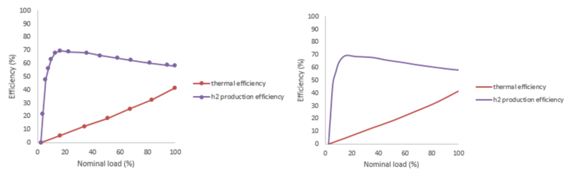
Fig.2: Piecewise and approximated efficiency of PEM electrolyzer.
Hydrogen and waste heat production
The maximum power of the electrolyzer, as defined by the user, is used to determine how much electricity is consumed at each load break point.
- \(bp_{el,H_{2},i}\) = ith hydrogen break point in terms of electricity consumption [Wh]
- \(bp_{load,H_{2},i}\) = ith hydrogen break point in terms of nominal load [-]
- \(bp_{el,th,i}\) = ith thermal break point in terms of electricity consumption [Wh]
- \(bp_{load,th,i}\) = ith thermal break point in terms of nominal load [-]
From these electricity consumption values, the absolute hydrogen and waste heat energy produced at each break point is calculated:
- \(H_{2_{prod,i}}\) = ith absolute hydrogen production value [kg]
- \(\mu_{H_{2},i}}\) = ith hydrogen production efficiency [-]
- \(E_{th,i}\) = ith absolute thermal energy value [Wh]
- \(\mu_{th,i}\) = ith thermal efficiency [-]
Piecewise Linear Transformer
The PEM electrolyzer component uses oemof’s Piecewise Linear Tansformer component in a similar fashion to the fuel cell CHP and the biogas CHP. For more detail on the usage, visit the Fuel Cell CHP or Gas Engine CHP Biogas components.
References
[1] Guo, Y. et.al. (2019). Comparison between hydrogen production by alkaline water electrolysis and hydrogen production by PEM electrolysis. IOP Conference Series: Earth and Environmental Science.
-
class
smooth.components.component_pem_electrolyzer.PemElectrolyzer(params)¶ Bases:
smooth.components.component.ComponentParameters: - name (str) – unique name given to PEM electrolyzer component
- bus_el (str) – electricity bus input of the PEM electrolyzer
- bus_h2 (str) – hydrogen bus output of the PEM electrolyzer
- bus_th (str) – thermal bus output of the PEM electrolyzer
- power_max (numerical) – maximum electrical input power [W]
- life_time (str) – life time of the component [a]
- set_parameters(params) (function) – updates parameter default values (see generic Component class)
- heating_value (numerical) – heating value of hydrogen [kWh/kg]
- bp_load_h2_prod (list) – hydrogen production efficiency load break points [-]
- bp_eff_h2_prod (list) – hydrogen production efficiency break points [-]
- bp_load_waste_heat (list) – waste heat efficiency load break points [-]
- bp_eff_waste_heat (list) – waste heat efficiency break points [-]
- bp_elec_consumed_h2_prod (list) – converted hydrogen production load points according to maximum power per timestep [Wh]
- bp_elec_consumed_waste_heat (list) – converted waste heat load points according to maximum power per timestep [Wh]
- bp_h2_production (list) – absolute hydrogen production values over the load points [kg]
- bp_waste_heat_energy – absolute waste heat energy values over the load points [Wh]
- bp_elec_consumed_h2_prod_half (list) – half the amount of electricity that is consumed [Wh]
- bp_elec_consumed_waste_heat_half – half the amount of electricity that is consumed [Wh]
- model_h2 (model) – hydrogen production model to set constraints later
- model_th (model) – waste heat model to set constraints later
-
add_to_oemof_model(busses, model)¶ Creates two separate oemof Piecewise Linear Transformer components for the hydrogen and waste heat production of the PEM electrolyzer from information given in the PEMElectrolyzer class, to be used in the oemof model
Parameters: - busses (dict) – virtual buses used in the energy system
- model (model) – oemof model containing the hydrogen production and waste heat production of the PEM electrolyzer
Returns: tuple of H2 and waste heat oemof components
-
get_h2_production_by_electricity(electricity_consumption)¶ Gets the hydrogen produced by the according electricity consumption value.
Parameters: electricity_consumption – electrcity consumption value [Wh] Returns: according hydrogen production value [kg]
-
get_waste_heat_energy_by_electricity(electricity_consumption)¶ Gets the waste heat produced by the according electricity consumption value.
Parameters: electricity_consumption – electrcity consumption value [Wh] Returns: according waste heat value [Wh]
-
update_constraints(busses, model_to_solve)¶ Set a constraint so that the electricity inflow of the hydrogen and the waste heat part are always the same (which is necessary while the piecewise linear transformer cannot have two outputs yet and therefore the two parts need to be separate components).
Parameters: - busses –
- model_to_solve –
Returns:
-
update_flows(results)¶ Updates the flows of the electrolyzer components for each time step.
::param results: The oemof results for the given time step :type results: object :return: updated flow values for each flow in the ‘flows’ dict
Power Converter
This module represents a generic power converter. It can be used to model AC-DC, DC-AC, AC-AC or DC-DC converters.
Scope
Power converters play an important role in diverse renewable energy systems, by regulating and shaping electrical signals in the appropriate forms for other components in the system and the demands.
Concept
A simple power converter component is created which intakes an AC or DC electric bus and transforms it into a different AC or DC electric bus with an assumed constant efficiency. The default efficiency is taken to be 95%, as stated in [1][2] for AC-DC converters. In [3] the efficiency for a DC-AC converter is given with 99%. This value should hence be modified by the user in the model definition. The amount of electricity that can leave the converter is limited by the defined maximum power.
Fig.1: Simple diagram of a power converter.
References
[1] Harrison, K.W. et. al. (2009). The Wind-to-Hydrogen Project: Operational Experience, Performance Testing, and Systems Integration, NREL. https://www.nrel.gov/docs/fy09osti/44082.pdf [2] Hayashi, Y. (2013). High Power Density Rectifier for Highly Efficient Future DC Distribution System, NTT Facilities Japan. [3] Sunny Highpower PEAK3 inverter (see manufacturer PDF)
-
class
smooth.components.component_power_converter.PowerConverter(params)¶ Bases:
smooth.components.component.ComponentParameters: - name (str) – unique name given to the AC-DC converter component
- bus_input (str) – electric input bus the converter is connected to
- bus_output (str) – electric output bus the converter is connected to
- output_power_max (numerical) – maximum output power [W]
- efficiency (numerical) – efficiency of the converter
-
add_to_oemof_model(busses, model)¶ Creates an oemof Transformer component using the information given in the PowerConverter class, to be used in the oemof model
Parameters: - busses (dict) – virtual buses used in the energy system
- model (oemof model) – current oemof model
Returns: oemof component
Sink
A generic sink component (usually for excess electricity, heat etc.) is created through this class.
Scope
A sink component is a virtual component that usually represents excesses in an energy system e.g. excess electricity or heat production.
Concept
The sink component is generic, where the input bus type and optionally the maximum input per time step are defined by the user. The default value is set to very high to represent a limitless capacity.
-
class
smooth.components.component_sink.Sink(params)¶ Bases:
smooth.components.component.ComponentParameters: - name (str) – unique name given to the sink component
- input_max (numerical) – maximum input per timestep of commodity e.g. for excess electricity [Wh], heat [Wh], hydrogen [kg]
- bus_in (str) – input bus of the sink component e.g. the electricity bus
- set_parameters(params) (function) – updates parameter default values (see generic Component class)
- commodity_costs (numerical) – costs for the commodities e.g. [EUR/Wh], [EUR/kg] (negative costs means the system earns money when the commodity enters the sink component)
-
add_to_oemof_model(busses, model)¶ Creates an oemof Sink component from the information given in the Sink class, to be used in the oemof model.
Parameters: - busses (dict) – virtual buses used in the energy system
- model (oemof model) – current oemof model
Returns: oemof component
Storage H2
This module represents a hydrogen storage tank.
Scope
Hydrogen can have a significant role in the integration of energy systems with its storage capabilities. By providing a capacity for storing excess electricity production, this can result in both the minimization of energy wasteage and smaller scale energy production systems whilst meeting the same demand. This is particularly important for cases of seasonal storage, where as an example, excess electricity production in the summer months with the lowest demands can be utilized at a later date.
Concept
The hydrogen storage component has a hydrogen bus input and a hydrogen bus output, which will sometimes be different from each other if another component in the system requires that the hydrogen has come directly from the storage, for instance.
Fig.1: Simple diagram of a hydrogen storage.
Initial storage level
The initial storage level is determined by the user through stating the capacity and the initial storage factor in relation to the capacity:
- \(SL_{init}\) = initial storage level [kg]
- \(F_{SL,init}\) = initial storage level as a factor of the capacity [-]
- \(C\) = storage capacity [kg]
Wanted storage level
It is optional for the user to define a wanted storage level through the storage level wanted factor (the default is set to None). If this value has been defined, then there will be different artificial costs used depending on whether the storage level is above or below the wanted level.
- \(SL_{wanted}\) = wanted storage level [kg]
- \(F_{SL,wanted}\) = wanted storage level as a factor of the capacity [-]
- \(C\) = storage capacity [kg]
Mass and volume
The minimum storage level mass at minimum pressure and the volume of the storage at maximum pressure are both calculated by initially using an iterative process where the specific volume is changed. First the initial value for the specific volume is given:
- \(V_{spec,0}\) = predfined initial value for specific volume [m³/mol]
Then using the initial value, the iterative process begins:
- \(V_{spec,i+1}\) = ith + 1 specific volume [m³/mol]
- \(R\) = gas constant [J/(K*mol)]
- \(T\) = storage temperature [K]
- \(p\) = storage pressure [Pa] (\(p_{min}\) for calculating the mass and \(p_{max}\) for the storage)
- \(rk_{a}\) = Redlich Kwong equation of state parameter a
- \(V_{spec,i}\) = ith specific volume [m³/mol]
- \(rk_{b}\) = Redlich Kwong equation of state parameter b
After ten iterations, the specific volume value is used to obtain the storage volume and the minimum storage level mass:
- \(V\) = storage volume [m³]
- \(C\) = storage capacity [kg]
- \(V_{spec}\) = specific volume [m³/mol]
- \(M_r\) = molar mass of H2 [kg/mol]
- \(SL_{min}\) = minimum storage level mass [kg]
Pressure
The pressure of the storage is calculated as follows:
- \(p\) = storage pressure [Pa]
- \(SL\) = storage level [kg]
-
class
smooth.components.component_storage_h2.StorageH2(params)¶ Bases:
smooth.components.component.ComponentParameters: - name (str) – unique name given to the storage component
- bus_in (str) – hydrogen bus that enters the storage
- bus_out (str) – hydrogen bus that leaves the storage
- p_min (numerical) – minimum pressure of the storage [bar]
- p_max (numerical) – maximum pressure of the storage [bar]
- storage_capacity (numerical) – storage capacity at maximum pressure (usable storage + minimum storage) [kg]
- life_time (numerical) – lifetime of the component [a]
- initial_storage_factor (numerical) – initial storage level as a factor of the capacity [-] e.g. 0.5 means half of the capacity
- delta_max (numerical) – maximum chargeable hydrogen in one time step [kg/t] where t is the step-size
- slw_factor (numerical) – storage level wanted as a factor of the capacity [-]
- vac_in (numerical) – normal variable artificial costs for charging (in) the storage [EUR/kg]
- vac_out (numerical) – normal variable artificial costs for discharging (out) the storage [EUR/kg]
- vac_low_in (numerical) – variable artificial costs for charging that apply if the storage level is below the wanted storage level [EUR/kg]
- vac_low_out (numerical) – variable artificial costs for discharging that apply if the storage level is below the wanted storage level [EUR/kg]
- set_parameters(params) (function) – updates parameter default values (see generic Component class)
- storage_level_init (numerical) – initial storage level [kg]
- T_crit (numerical) – critical temperature [K]
- p_crit (numerical) – critical pressure [Pa]
- Mr (numerical) – molar mass of H2 [kg/mol]
- R – gas constant [J/(K*mol)]
- rk_a (numerical) – Redlich Kwong equation of state parameter a
- rk_b (numerical) – Redlich Kwong equation of state parameter b
- V (numerical) – storage volume [m³]
- storage_level_min (numerical) – mass at minimum pressure that can’t be used [kg]
- storage_level (numerical) – storage level [kg]
- pressure (numerical) – storage pressure [bar]
- current_vac (list) – current artificial costs for input and output [EUR/kg]
-
add_to_oemof_model(busses, model)¶ Creates an oemof Generic Storage component from the information given in the StorageH2 class, to be used in the oemof model.
Parameters: - busses (dict) – virtual buses used in the energy system
- model (oemof model) – current oemof model
Returns: oemof component
-
get_mass(p, V=None)¶ Calculates the mass of the storage at a certain pressure.
Parameters: - p (numerical) – pressure [bar]
- V (numerical) – storage volume [m³]
Returns: mass of the storage [kg]
-
get_pressure(m)¶ Calculates the storage pressure for a given mass.
Parameters: m (numerical) – mass [kg] Returns: pressure [bar]
-
get_volume(p, m)¶ Calculates the volume needed to fit a certain mass at given pressure.
Parameters: - p (numerical) – pressure [bar]
- m (numerical) – mass [kg]
Returns: volume of the storage [m³]
-
prepare_simulation(components)¶ Prepares the simulation by setting the appropriate artificial costs and the maximum chargeable hydrogen in one time step (delta max).
Parameters: components (list) – List containing each component object Returns: artificial costs and delta max
-
update_states(results)¶ Updates the states of the storage component for each time step
Parameters: results (object) – oemof results for the given time step Returns: updated state values for each state in the ‘state’ dict
Stratified Thermal Storage
This module represents a stratified thermal storage tank, based on oemof thermal’s component.
Scope
A stratified thermal storage vessel is able to store thermal energy through stratification, and thus minimise energy wastage in systems.
Concept
This component has been largely based on oemof thermal’s stratified thermal storage component. Visit oemof thermal’s readthedocs site for detailed information on how the component was constructed [1].
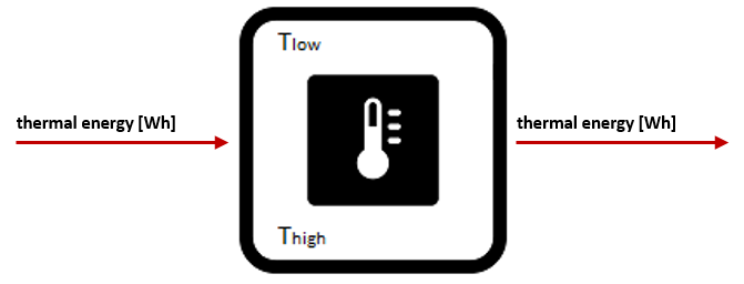
Fig.1: Simple diagram of an electric heater.
References
- [1] oemof thermal (2019). Stratified thermal storage, Read the Docs:
- https://oemof-thermal.readthedocs.io/en/latest/stratified_thermal_storage.html
-
class
smooth.components.component_stratified_thermal_storage.StratifiedThermalStorage(params)¶ Bases:
smooth.components.component.ComponentParameters: - name (str) – unique name given to the stratified thermal storage component
- bus_in (str) – thermal bus input of the storage
- bus_out (str) – thermal bus output of the storage
- storage_capacity (numerical) – storage capacity [Wh]
- storage_level_min (numerical) – minimum storage level relative to storage capacity [-]
- storage_level_max (numerical) – maximum storage level relative to storage capacity [-]
- max_heat_flow_charge (numerical) – maximum heat charged into the storage per timestep [Wh]
- max_heat_flow_discharge (numerical) – maximum heat discharged from the storage per timestep [Wh]
- storage_level_init (numerical) – initial storage level [Wh]
- life_time (numerical) – lifetime of the component [a]
- nominal_value (numerical) – value that the timeseries should be multipled by, default is 1
- csv_filename – csv filename containing the desired demand timeseries
- csv_separator (str) – separator of the csv file e.g. ‘,’ or ‘;’, default is ‘,’
- column_title (str or int) – column title (or index) of the timeseries, default is 0
- path (str) – path where the timeseries csv file can be located
- density (numerical) – density of the storage medium [kg/m3]
- heat_capacity (numerical) – heat capacity of the storage medium [J/(kg*K)]
- temp_h (numerical) – hot temperature level of the stratified storage tank [K]
- temp_c (numerical) – cold temperature level of the stratified storage tank [K]
- temp_env (numerical) – environment temperature value [C] because timeseries usually in degrees C
- height_diameter_ratio (numerical) – height to diameter ratio of storage tank [-]
- s_iso (numerical) – thickness of isolation layer [m]
- lamb_iso (numerical) – heat conductivity of isolation material [W/(m*K)]
- alpha_inside (numerical) – heat transfer coefficient inside [W/(m2*K)]
- alpha_outside (numerical) – heat transfer coefficient outside [W/(m2*K)]
- vac_in (numerical) – normal var. art. costs for charging in the storage [EUR/Wh]
- vac_out (numerical) – normal var. art. costs for discharging out the storage [EUR/Wh]
- storage_level_wanted (numerical) – if a storage level is set as wanted, the vac_low costs apply if the storage is below that level [Wh].
- vac_low_in (numerical) – var. art. costs that apply if storage level is below wanted storage level [Wh]
- vac_low_out (numerical) – var. art. costs that apply if storage level is below wanted storage level [Wh]
- set_parameters(params) (function) – updates parameter default values (see generic Component class)
- storage_level (numerical) – storage level [Wh]
- current_vac (array) – stores the current artificial costs for input and output [EUR/Wh]
- volume (numerical) – storage volume [m³]
- diameter (numerical) – diameter of the storage [m]
- u_value (numerical) – thermal transmittance [W/(m2*K)]
- loss_rate (numerical (sequence or scalar)) – relative loss of the storage capacity between two consecutive timesteps [-]
- fixed_losses_relative (numerical (sequence or scalar)) – losses independent of state of charge between two consecutive timesteps relative to nominal storage capacity [-]
- fixed_losses_absolute (numerical (sequence or scalar)) – losses independent of state of charge and independent of nominal storage capacity between two consecutive timesteps [Wh]
-
add_to_oemof_model(busses, model)¶ Creates an oemof GenericStorage component from the information given in the Stratified Thermal Storage class, to be used in the oemof model
Parameters: - busses (dict) – virtual buses used in the energy system
- model (oemof model) – current oemof model
Returns: oemof component
-
calculate_losses(u_val, d, de, h_c, t_c, t_h, t_env, time_increment=1)¶ Calculates the loss rate and the fixed losses for the stratified thermal storage
Parameters: - u_val (numerical) – thermal transmittance [W/(m2*K)]
- d (numerical) – diameter of storage tank [m]
- de (numerical) – density of the storage medium [kg/m3]
- h_c (numerical) – heat capacity of storage medium [J/(kg*K)]
- t_c (numerical) – cold temperature level of the stratified storage tank [K]
- t_h (numerical) – hot temperature level of the stratified storage tank [K]
- t_env (numerical (sequence or scalar)) – environmental temperature [K]
- time_increment (numerical) – time increment of the oemof.solph.EnergySytem [h]
Returns: loss rate, relative fixed losses and absolute fixed losses
-
calculate_storage_u_value(a_in, s_iso, l_iso, a_out)¶ Calculates the u value (thermal transmittance) of storage envelope
Parameters: - a_in (numerical) – heat transfer coefficient inside [W/(m2*K)]
- s_iso (numerical) – thickness of isolation layer [m]
- l_iso (numerical) – heat conductivity of isolation material [W/(m*K)]
- a_out (numerical) – heat transfer coefficient outside [W/(m2*K)]
Returns: u value
-
get_diameter(V, h_d_ratio)¶ Calculates the diameter of the storage tank
Parameters: - V (numerical) – storage tank volume [m3]
- h_d_ratio (numerical) – height to diameter ratio of storage tank [-]
Returns: storage tank diameter
-
get_volume(s_c, h_c, de, t_h, t_c)¶ Calculates the storage tank volume
Parameters: - s_c (numerical) – storage capacity [Wh]
- h_c (numerical) – heat capacity of storage medium [J/(kg*K)]
- de (numerical) – density of the storage medium [kg/m3]
- t_h (numerical) – hot temperature level of the stratified storage tank [K]
- t_c (numerical) – cold temperature level of the stratified storage tank [K]
Returns: storage tank volume
-
prepare_simulation(components)¶ Prepares the simulation by applying the appropriate variable artificial costs
Parameters: components (list) – List containing each component object Returns: array containing var. art. costs in and out of the storage
-
update_states(results)¶ Updates the states of the thermal storage component for each time step
Parameters: results (object) – oemof results for the given time step Returns: updated state values for each state in the ‘state’ dict
Supply
A generic supply component (usually for grid supplied electricity, heat etc.) is created through this class.
Scope
A supply component is a generic component that represents a supply to the energy system such as an electricity grid or a hydrogen grid.
Concept
The output bus type and the maximum output per timestep are defined by the user, and similarly to in the sink component, the default maximum output value is set to very high to represent a limitless capacity.
Artificial costs
There are some energy systems where the supply component should be incentivised to be used in certain scenarios and not in others. As an example, an energy system with renewable energy electricity production, the electricity grid as an alternative supply and hydrogen production/storage is considered.
If the hydrogen storage is over a defined threshold, then the system wants to prioritise using the stored hydrogen as an energy source instead of extracting energy from the grid, which is achieved by setting high artificial costs on the use of the grid component. If the hydrogen storage is below the defined threshold, however, then the system is incentivised to use the grid so that the storage does not entirely run out.
-
class
smooth.components.component_supply.Supply(params)¶ Bases:
smooth.components.component.ComponentParameters: - name (str) – unique name given to the supply component
- output_max (numerical) – maximum output per timestep of commodity e.g. for the electricity grid [Wh], thermal grid [Wh], H2 grid [kg/h]
- bus_out (str) – output bus of the supply component e.g. the electricity bus
- fs_threshold (numerical) – threshold value for artificial costs
- fs_low_art_cost (numerical) – low artificial cost value e.g. [EUR/Wh], [EUR/kg]
- fs_high_art_cost (numerical) – high artificial cost value e.g. [EUR/Wh], [EUR/kg]
- fs_pressure (numerical) – pressure of the supply if required (default is None) [bar]
- set_parameters(params) (function) – updates parameter default values (see generic Component class)
- current_ac (numerical) – current artificial cost value e.g. [EUR/Wh], [EUR/kg]
-
add_to_oemof_model(busses, model)¶ Creates an oemof Source component from the information given in the Supply class, to be used in the oemof model.
Parameters: - busses (dict) – virtual buses used in the energy system
- model (oemof model) – current oemof model
Returns: oemof component
-
prepare_simulation(components)¶ Prepares the simulation by updating the artificial costs for the current time step (dependant on foreign states) and sets the total costs for the commodity for this time step (costs + artificial costs)
Parameters: components (list) – List containing each component object Returns: total costs for the commodity for this time step e.g. [EUR/Wh], [EUR/kg]
Trailer Gate
A trailer gate component is created to limit the flows into the trailer component depending on whether delivery is possible or not.
Scope
The trailer gate component is a virtual component, so would not be found in a real life energy system, but is used in parallel with the trailer components to restrict the flows into the trailers depending on if delivery is possible or not.
Concept
A transformer component is used with a hydrogen bus input and a hydrogen bus output, where the hydrogen bus input comes from e.g. the production site and the hydrogen bus output goes to the trailer. The flow of hydrogen allowed to enter the trailer is controlled by the flow switch and whether delivery is possible in the given timestep or not.
-
class
smooth.components.component_trailer_gate.TrailerGate(params)¶ Bases:
smooth.components.component.ComponentParameters: - name (str) – unique name given to the trailer gate component
- max_input (numerical) – maximum mass of hydrogen that can flow into the component [kg]
- trailer_distance (numerical) – distance for trailer delivery [km]
- driver_costs (numerical) – driver costs [EUR/h]
- bus_in (numerical) – input hydrogen bus [kg]
- bus_out (numerical) – output hydrogen bus [kg]
- round_trip_distance (numerical) – round trip distance from origin to destination [km]
- set_parameters(params) (function) – updates parameter default values (see generic Component class)
- flow_switch (int) – determines whether there is a flow in the current timestep: 0 = off, 1 = on
-
add_to_oemof_model(busses, model)¶ Creates an oemof Transformer component from the information given in the TrailerGate class, to be used in the oemof model.
Parameters: - busses (dict) – virtual buses used in the energy system
- model (oemof model) – current oemof model
Returns: oemof component
-
prepare_simulation(components)¶ Updates artificial costs for this time step (dependent on foreign states) and determines the maximum hydrogen input for the component.
Parameters: components (list) – List containing each component object Returns: artificial costs and maximum allowed hydrogen input
-
update_var_costs()¶ Calculates variable costs of the component which only applies if the trailer is used, based on the distance travelled by the trailer.
Trailer Gate Cascade
A cascade trailer gate component is created to control the output flows from a trailer delivery to a destination site.
Scope
Similarly to the other gate components, the cascade trailer gate component is virtual and would not be found in a real life energy system. This component is used in parallel with the trailer cascade component to control how hydrogen is distributed between destination sites in the same trip.
Concept
A transformer component is used with a hydrogen bus input and a hydrogen bus output, where the hydrogen is inputted from the trailer and outputted to the destination site. The amount of hydrogen that can be delivered to the destination site is restricted by the maximum input value that is determined in the cascade trailer component. Notably, a different gate component should be created for each destination site.
-
class
smooth.components.component_trailer_gate_cascade.TrailerGateCascade(params)¶ Bases:
smooth.components.component.ComponentParameters: - name (str) – unique name given to the cascade trailer gate component
- max_input (numerical) – maximum mass of hydrogen that can flow into the component [kg]
- bus_in (numerical) – input hydrogen bus [kg]
- bus_out (numerical) – output hydrogen bus [kg]
- set_parameters(params) (function) – updates parameter default values (see generic Component class)
-
add_to_oemof_model(busses, model)¶ Creates an oemof Transformer component from the information given in the TrailerGateCascade class, to be used in the oemof model.
Parameters: - busses (dict) – virtual buses used in the energy system
- model (oemof model) – current oemof model
Returns: oemof component
-
prepare_simulation(components)¶ Sets the maximum input of the component by using the value calculated in the cascade trailer component as a foreign state.
Parameters: components (list) – List containing each component object Returns: maximum allowed hydrogen input
Trailer H2 Delivery
This module represents a hydrogen trailer delivery from multiple production sites.
Scope
Hydrogen trailers can be crucial in an energy system as a means of transporting hydrogen from the production site to the destination site (e.g. a refuelling station).
Concept
The hydrogen trailer component is a transformer component with a hydrogen bus input and a hydrogen bus output, which should be distinct from each other in order to maintain a one way flow from the production site to the destination site.
Fig.1: Simple diagram of a hydrogen delivery trailer
This component should be used in parallel with the trailer gate component. The amount of hydrogen that can be transported in a given time step is determined, and this value restricts the flow in the component. A simple depiction of how the concept for the single hydrogen delivery trailer is shown in Figure 2.
Fig.2: Multiple hydrogen delivery trailer concept
Trailer activity
In this component, the trailer has the option of transporting hydrogen from multiple production sites to one destination. Thresholds are set for both the origin and destination storages. The component then:
- Checks the level of destination storage component: if it is below specified threshold, low artificial costs are implemented (to encourage system to fill it).
- Checks the level of the origin storage components and chooses the one with maximum available mass of hydrogen
- Takes into consideration the mass of hydrogen in the chosen origin storage component and the destination storage, as well as the trailer capacity, and transports the maximum possible amount of hydrogen.
- Considers the round trip distance along with the assumptions that the trailer can travel at 100 km/h and that the refuelling time for the trailer is 15 minutes. With this information, it is determined whether or not delivery is possible for the following time step with the trailer.
-
class
smooth.components.component_trailer_h2_delivery.TrailerH2Delivery(params)¶ Bases:
smooth.components.component.ComponentParameters: - name (str) – unique name given to the trailer components
- bus_in (str) – input hydrogen bus to the trailer
- bus_out (str) – output hydrogen bus from the trailer
- trailer_capacity (numerical) – trailer capacity [kg]
- fs_destination_storage_threshold (numerical) – threshold for destination storage to encourage/discourage the use of the trailer [-]
- hydrogen_needed (numerical) – mass of hydrogen needed from delivery [kg]
- fs_origin_available_kg (numerical) – foreign state for the available mass of hydrogen in the origin storage [kg]
- set_parameters(params) (function) – updates parameter default values (see generic Component class)
- current_ac (numerical) – current artificial cost value [EUR/kg]
-
add_to_oemof_model(busses, model)¶ Creates an oemof Transformer component from the information given in the TrailerH2Delivery class, to be used in the oemof model.
Parameters: - busses (dict) – virtual buses used in the energy system
- model (oemof model) – current oemof model
Returns: oemof component
-
prepare_simulation(components)¶ Prepares the simulation by determining trailer activity such as which origin storage to take from and how much hydrogen is needed.
Parameters: components (list) – List containing each component object Returns: artificial costs and amount of hydrogen needed
Trailer H2 Delivery Cascade
This module represents a hydrogen trailer delivery from a single production site to one main destination site, and a secondary destination site that is dependent on the main site when necessary.
Scope
Hydrogen trailers can be crucial in an energy system as a means of transporting hydrogen from the production site to the destination site (e.g. a refuelling station). Sometimes it is the case that one production site should supply hydrogen to destination sites that are in close proximity to each other, for instance. If this is the case, it is beneficial for the energy system productivity to supply to both storages in one trip. This component represents a case where there is one main destination site that needs regular delivery, and one secondary destination site that will receive a delivery in the same trip as to the main destination site when necessary.
Concept
The cascade hydrogen trailer component is also a transformer component with a hydrogen bus input and output that are distinct from each other. This component should be used in parallel with the trailer gate and trailer gate cascade components. The amount of hydrogen that can be transported in a given time step is determined, and this value restricts the flow in the component.
Fig.1: Simple diagram of a hydrogen delivery trailer
A simple depiction of the concept for the single hydrogen delivery trailer is shown in Figure 2.
Fig.2: Cascade hydrogen delivery trailer concept
Trailer activity
In this component, the trailer has the option of transporting hydrogen from one production site to two destination sites that are dependent on one another. Thresholds are set for the origin and destination storages. The component then:
- Checks the level of the origin storage component: if it is below specified threshold, the trailer cannot take hydrogen from it.
- Checks the level of destination storage components: if they are both below their specified thresholds, then the trailer is incentivised to deliver to both storages.
- Checks the mass of hydrogen in all storages as well as the trailer capacity, and transports the maximum possible amount of hydrogen.
- Calculates how much hydrogen should get delivered to the main and secondary destination storages, prioritising filling up the main storage when necessary.
-
class
smooth.components.component_trailer_h2_delivery_cascade.TrailerH2DeliveryCascade(params)¶ Bases:
smooth.components.component.ComponentParameters: - name (str) – unique name given to the trailer component
- bus_in (str) – input hydrogen bus to the trailer
- bus_out (str) – output hydrogen bus from the trailer
- trailer_capacity (numerical) – trailer capacity [kg]
- fs_destination_storage_threshold_1 (numerical) – threshold for main destination storage to encourage/discourage the use of the trailer [-]
- fs_destination_storage_threshold_2 (numerical) – threshold for secondary destination storage to encourage/discourage delivery to it [-]
- hydrogen_needed (numerical) – mass of hydrogen needed from delivery [kg]
- output_h2_1 – amount of hydrogen delivered to main destination [kg]
- output_h2_2 – amount of hydrogen delivered to secondary destination [kg]
- fs_origin_available_kg (numerical) – foreign state for the available mass of hydrogen in the origin storage [kg]
- set_parameters(params) (function) – updates parameter default values (see generic Component class)
- current_ac (numerical) – current artificial cost value [EUR/kg]
-
add_to_oemof_model(busses, model)¶ Creates an oemof Transformer component from the information given in the TrailerH2DeliveryCascade class, to be used in the oemof model.
Parameters: - busses (dict) – virtual buses used in the energy system
- model (oemof model) – current oemof model
Returns: oemof component
-
prepare_simulation(components)¶ Prepares the simulation by determining trailer activity and parameters such as how much hydrogen is needed for delivery and how this should be distributed between the destination storages.
Parameters: components (list) – List containing each component object Returns: artificial costs, amount of hydrogen needed and the amounts delivered to each storage
Trailer H2 Delivery Single
This module represents a hydrogen trailer delivery from a single production site.
Scope
Hydrogen trailers can be crucial in an energy system as a means of transporting hydrogen from the production site to the destination site (e.g. a refuelling station).
Concept
Similarly to the hydrogen trailer component with multiple production sites, the single hydrogen trailer component is a transformer component with a hydrogen bus input and a hydrogen bus output, which should be distinct from each other in order to maintain a one way flow from the production site to the destination site.
Fig.1: Simple diagram of a hydrogen delivery trailer
The only difference between this component and the hydrogen trailer component is that here, there is only one option for the origin storage and this is predetermined. This component should be used in parallel with the trailer gate component. The amount of hydrogen that can be transported in a given time step is determined, and this value restricts the flow in the component. A simple depiction of how the concept for the single hydrogen delivery trailer is shown in Figure 2.

Fig.2: Single hydrogen delivery trailer concept
Trailer activity
Thresholds are set for both the origin and destination storages. The component then:
- Checks the level of destination storage component: if it is below specified threshold, low artificial costs are implemented (to encourage system to fill it).
- Checks the level of origin storage component: if it is below specified threshold, the trailer cannot take any hydrogen from it.
- Checks the mass of hydrogen in both storages along with taking the trailer capacity into consideration, and transports the maximum possible amount of hydrogen.
- Considers the round trip distance along with the assumptions that the trailer can travel at 100 km/h and that the refuelling time for the trailer is 15 minutes. With this information, it is determined whether or not delivery is possible for the following time step with the trailer.
-
class
smooth.components.component_trailer_h2_delivery_single.TrailerH2DeliverySingle(params)¶ Bases:
smooth.components.component.ComponentParameters: - name (str) – unqiue name given to the trailer component
- bus_in (str) – input hydrogen bus to the trailer
- bus_out (str) – output hydrogen bus from the trailer
- trailer_capacity (numerical) – trailer capacity [kg]
- fs_destination_storage_threshold (numerical) – threshold for destination storage to encourage/discourage the use of the trailer [-]
- hydrogen_needed (numerical) – mass of hydrogen needed from delivery [kg]
- fs_origin_available_kg (numerical) – foreign state for the available mass of hydrogen in the origin storage [kg]
- set_parameters(params) (function) – updates parameter default values (see generic Component class)
- current_ac (numerical) – current artificial cost value [EUR/kg]
-
add_to_oemof_model(busses, model)¶ Creates an oemof Transformer component from the information given in the TrailerH2DeliverySingle class, to be used in the oemof model.
Parameters: - busses (dict) – virtual buses used in the energy system
- model (oemof model) – current oemof model
Returns: oemof component
-
prepare_simulation(components)¶ Prepares the simulation by determining trailer activity and how much hydrogen is needed
Parameters: components (list) – List containing each component object Returns: artificial costs and the amount of hydrogen needed
Variable Grid
-
class
smooth.components.component_var_grid.VarGrid(params)¶ Bases:
smooth.components.component_supply.SupplyAn electric grid with different connection levels can be created through this class
Gridlevels [1,2,3,4,5,6] describe the grid connection, if left unmodified these are: [1] house connection, [2] lov voltage grid, [3] lov voltage local network station [4] medium voltage grid, [5] medium voltage transformer station, [6] High Voltage. These can be associated with different output_max, variable costs, capex and opex for each level.Parameters: - self.name (str) – unique name of the component
- self.grid_level (int (1-6)) – set the grid level to be used
- self.grid_l1_output_max (int) – Maximum power output of specific grid level [W]
- self.capex_l1 (dict) – Capex for each grid level (e.g grid connection costs)
- self.opex_l1 (dict) – Opex for each grid level (e.g grid maintanance costs)
- self.variable_costs_l1 (numerical) – Variable costs for each grid level (e.g electricity costs)
External Components
This class is created for external components in the system that will not be part of the optimization, but the CAPEX and OPEX of these components should still be evaluated.
Scope
External components are used in the framework to represent components that do not need to be included in the simulation/optimization, but nevertheless the annuities in terms of costs and emissions for the component should be considered. The generic ExternalComponent class is the mother class for the other external components, providing a basis for what all external components must have.
Concept
The costs (CAPEX and OPEX) and emissions of the external component are first calculated
(see the update_financials() and
update_emissions() functions), and
then the annuities are calculated using the
update_external_annuities() function.
It should be noted that these costs are not considered in the optimization results as
they are evaluated seperately.
-
class
smooth.components.external_component.ExternalComponent¶ Bases:
objectParameters: - external_component (str) – external component type
- name (str) – specific name of the external component (must be unique)
- life_time (numerical) – lifetime of the external component [a]
- sim_params (object) – simulation parameters such as the interval time and interest rate
- results (dict) – dictionary containing the main results for the component
- capex (dict) – capital costs
- opex (dict) – operational and maintenance costs
- op_emissions (dict) – operational emission values
- fix_emissions (dict) – fixed emission values
-
check_validity()¶ This function is called immediately after the component object is created and checks if the component attributes are valid.
Raises: ValueError – Value error raised if the life time is not defined or is less than or equal to 0
-
generate_results()¶ Generates the results after the simulation.
Returns: Results for the calculated emissions, financials and annuities
-
set_parameters(params)¶ Sets the parameters that have been defined by the user (in the model definition) in the necessary components, overwriting the default parameter values.
Parameters: params (dict ToDo: make sure of this, maybe list) – The set of parameters defined in the specific external component class Raises: ValueError – raised if the parameter defined by the user is not part of the external component Returns: None
H2 Dispenser
This external component class is created to represent the dispenser unit of a hydrogen refuelling station.
Scope
The dispenser unit of a hydrogen refuelling station does not need to be included in the optimization of an energy system, as the number of units necessary can be calculated from the hydrogen demand, but the costs of the dispensers should be considered in the final evaluation of the energy system.
Concept
This component requires a demand time series in the form of a CSV file. From this file, the maximum hydrogen demand in one time step is found. Then, the number of times each hose can refuel a vehicle per hour is calculated, as well as the maximum number of vehicles that require refuelling per hour. The number of dispenser units required is then calculated as follows:
- \(U\) = number of dispenser units required [-]
- \(V_{max}\) = maximum number of vehicles that need refuelling in an hour [-]
- \(H\) = number of hoses per dispenser [-]
- \(R\) = number of possible refuels per hour [-]
-
class
smooth.components.external_component_h2_dispenser.H2Dispenser(params)¶ Bases:
smooth.components.external_component.ExternalComponentParameters: - name (str) – unique name given to the H2 dispenser component
- life_time (numerical) – life time of the component [a]
- vehicle_tank_size (numerical) – vehicle tank size - 40 kg for a bus and 5 kg for a passenger car are used as default [kg]
- number_of_hoses (int) – number of hoses (access points) attached to the dispenser - default is set to 2 [-]
- refuelling_time (numerical) – refuelling time to fill up the specified tank [min] - default is set to 15
- nominal_value (numerical) – value that the timeseries should be multipled by, default is 1
- csv_filename – csv filename containing the desired demand timeseries e.g. ‘my_demand_filename.csv’
- csv_separator (str) – separator of the csv file e.g. ‘,’ or ‘;’, default is ‘,’
- column_title (str or int) – column title (or index) of the timeseries, default is 0
- path (str) – path where the timeseries csv file can be located
- set_parameters(params) (function) – updates parameter default values (see generic Component class)
- data (pandas dataframe) – dataframe containing data from timeseries
- max_hourly_h2_demand (numerical) – maximum value per timestep
- number_of_refuels_per_hour (numerical) – number of times each hose can refuel a vehicle per hour
- max_number_of_vehicles (numerical) – maximum amount of vehicles that need refuelling per hour
- number_of_units (numerical) – number of dispenser units required in order to satisfy the demand